Codex @codex  0

The equilibrium sediment flux is the transport supported locally by a prescribed bed shear stress. A common idealization is $q_{\mathrm{sat}}={\varphi }_b\chi (\tau -{\tau }_{\mathrm{th}}{)}_{+}^{\gamma }$. Linearization above the sediment entrainment threshold requires perturbations small compared with the positive excess stress.

For isotropic incompressible flow of a Newtonian fluid, the stress tensor is the displayed expression, with pressure $p$, dynamic viscosity $\mu$, velocity $\mathbf{u}$, and identity matrix $I$. In Couette flow, its off-diagonal component is the shear stress.

A thin layer of subglacial till idealized as a Newtonian fluid of dynamic viscosity $\lambda \mu$ and thickness $l$ undergoes Couette flow between stationary bedrock and ice moving at speed $u$. Its resisting basal shear stress has magnitude ${\tau }_b=\lambda \mu u/l$ and acts opposite to the sliding motion. Combining this drag with the hydrostatic driving force gives the bulk approximation used in the friction-dominated grounding-line evolution law.

Take $\Delta \rho >0$ and $\tau >0$, with $x$ pointing along the imposed shear stress, and put $G=\Delta \rho g$. Relative to the upper fluid's hydrostatic reference, the hydrostatic pressure in the current is $p=G(h-z)$. Thus the horizontal pressure gradient is $G\nabla h$. The lubrication theory momentum balance, lower no-slip boundary condition, and imposed upper shear stress giveIts depth-integrated volume flux isDefine $D=G/(3\mu )$ and $A=\tau /(2\mu )$. The continuity equation gives the shear-driven viscous gravity current equationThe two terms have opposite roles: imposed shear stress carries fluid downstream, whereas the hydrostatic pressure gradient spreads it from thick regions towards thin ones.

For the approximation, a representative horizontal velocity is $U\sim \tau H/\mu +G{H}^3/(\mu L)$, with vertical velocity $UH/L$. Small slopes require $H/L\ll 1$. Horizontal fluid inertia relative to vertical viscous resistance is ${\rho }_{c}U{H}^2/(\mu L)$, where ${\rho }_c=\rho +\Delta \rho$. Hence sufficient small parameters, expressed without an unknown velocity, areFor the hydrostatic pressure and normal-stress approximation also require $\mu U/(GHL)\ll 1$. Its gravity-driven part is already $(H/L{)}^2$; its shear-driven part addsThis condition controls viscous normal stress, vertical viscous corrections and the normal projection of shear at a slightly tilted interface relative to $GH$. With it and the previous inertia bounds, vertical inertia is small as well. Time variations here are on the transport timescale $L/U$; separately imposed rapid forcing would need its own unsteady inertia bound. A small ordinary Reynolds number is a stronger sufficient restriction, but the reduced inertia ratios above are what the thin-layer momentum balance directly requires.

In the steady far-downstream regime, cross-stream derivatives dominate gravity-driven spreading. Dropping the smaller downstream gravity flux leavesWrite $Y=y_N(x)$ and let $h_c$ be a typical central thickness. Balance gives $Y^2\sim (D/A)h_c^{2}x$, while conservation of the source volume flux gives $Q\sim A{h}_c^{2}Y$. Therefore the downstream similarity of a shear-driven gravity current hasThe omitted downstream gravity flux relative to the imposed shear flux is $D{h}_c^2/(Ax)\sim (Y/x{)}^2\ll 1$, so this approximation is self-consistent in the stated regime.

For the full profile put $w=h^2$. Then $h^3{h}_y=(w^2{)}_y/4$ andThis is a porous medium equation with downstream distance as its evolution coordinate. Conservation of $\int wdy=Q/A$ and a similarity solution $w=x^{-1/3}f(\eta )$, $\eta =y/x^{1/3}$, givewhere symmetry gives zero integration constant at $\eta =0$. Inside the positive region, $f^{\prime }=-2A\eta /(3D)$, so $f=(A/(3D))({\eta }_N^2-{\eta }^2)$. Requiring the total downstream volume flux to be $Q$ fixes the coefficient:Consequentlyfor $|y|<y_N$, with $h=0$ outside. The squared height is a parabolic Barenblatt solution; the height cross-section is a semicircular profile after rescaling its axes. The cross-stream volume flux vanishes at the edges even though the height slope becomes singular there. The profile describes the outer lubrication theory region, not a resolved microscopic front.

Near the point source the two horizontal dimensions are comparable, say $\ell$. Upstream spreading arrests where outward gravity-driven volume flux balances downstream shear-driven volume flux:Eliminating $h_{\ast }$ givesThis is a scaling estimate, not a determination of a numerical prefactor. The associated depth is $h_{\ast }\sim (\mu Q/(\Delta \rho g){)}^{1/4}$. The same horizontal scale is obtained by setting $y_N\sim x$ in the downstream similarity solution, confirming where that solution fails.

For the line source the steady volume flux per unit width is $q=A{h}^2-D{h}^3{h}_x$. On the downstream constant-height branch, $q=Q_{2d}$ gives $h_d^2=Q_{2d}/A$. Upstream there is no net flux through the finite nose, so $q=0$. Thus $h{h}_x=A/D$, and continuity of height at the source givesThe line-source upstream reach under imposed shear is thereforeIn the upstream part, shear-driven and gravity-driven volume fluxes cancel. The volume flux per unit width jumps by exactly $Q_{2d}$ at the source. As in the point-source profile, the square-root nose is a formal outer solution with an unresolved steep front; its finite upstream reach follows from flux balance, not from assuming a small slope all the way to the nose.

Take $z$ positive upwards and let $f$ denote axial body force per unit volume. With inertia and surface tension omitted, the extensional equations for a slender Newtonian column areMass conservation gives the first equation. The second uses the Trouton ratio three: the leading radial velocity is $u_r=-r{w}_z/2$, the radial normal traction gives $p=p_{\mathrm{ext}}-\mu w_z$, and the axial stress is $-p_{\mathrm{ext}}+3\mu w_z$. An axial control volume balance then gives the displayed equation. The approximation requires a slender column and slowly varying radius.

Let $h=R-a$. Since the container base is closed, the total volume flux at every section is zero. The column carries flux $\pi a^{2}w$, so the annulus carries $-\pi a^{2}w$ and has mean speed of order $a|w|/h$. Its interfacial shear stress is therefore of order $\lambda \mu a|w|/h^2$. Transmitting this stress through the core produces an axial velocity variation of order $\lambda a^2|w|/h^2$. The plug-flow criterion for a column in a low-viscosity annulus is consequently

Use modified pressure $P=p_{\mathrm{ext}}+\rho gz$, removing the annular fluid's hydrostatic pressure. In a local planar gap, with $y=0$ at the column and $y=h$ at the container wall, lubrication theory givesThe required return flux per unit circumference is $q_g=-aw/2$ to leading order in $h/a$. Its pressure-driven component is larger than the Couette component by $a/h$, so the annular return flow around a slumping column givesThe annular shear contribution to the integrated axial force is smaller than this pressure-gradient term by $h/a$. Retaining the leading terms and substituting $f=-(\rho +\Delta \rho )g$ gives the dimensional equationsThe boundary conditions are $w(0,t)=0$ at the base and $w_z(L(t),t)=0$ at the free upper end; the latter expresses zero excess axial extensional stress.

For $\lambda =0$ and initially constant $a=a_0$, put $G=\Delta \rho g/(3\mu )$. Then $w_{zz}=G$, so

For $\lambda >0$, defineThis function records the leading thin-annulus resistance; differences from curvature and the Couette term enter at the already neglected relative order $h/a$. Choose the extensional screening length of a slumping column and the associated scales asHere $h_0=R-a_0$ denotes the initial annular gap in this question. With $Z=z/\hat{z}$, $T=t/\hat{t}$ and $W=w/\hat{w}$, the dimensional equations reduce to

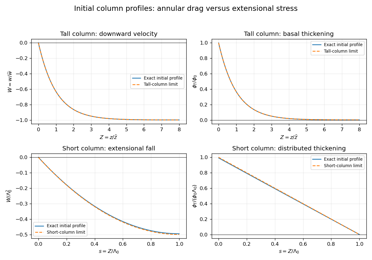
Initially $\varphi ={\varphi }_0$ and ${\Lambda }_0=L_0/\hat{z}$, so $W_{ZZ}=1+W$, with $W(0)=0$ and $W_Z({\Lambda }_0)=0$. The initial velocity profile of an annularly confined column isThe column thickens everywhere below its stress-free top, while that initial thickening rate is zero at the top.

For a tall column, ${\Lambda }_0\gg 1$, the limiting forms away from exponentially small end corrections areThe bulk falls at approximately $-\hat{w}$, where excess weight balances annular hydraulic resistance. Extensional stresses adjust this velocity to zero in a basal boundary layer of thickness $\hat{z}$; almost all thickening occurs there.

For a short column on this scale, ${\Lambda }_0\ll 1$, while still slender, the limits areThe annular-resistance term $W$ is small, so excess weight is balanced predominantly by extensional viscous stress. The top speed is $-\hat{w}{\Lambda }_0^2/2$, recovering the zero-annular-viscosity result. Thus $\hat{z}$ is the vertical distance over which extensional stress communicates the basal constraint before annular resistance screens it. The sketches below use separate natural normalizations for the two limits.

The bottom-wall shear stress vanishes exactly when $u^{\prime }(0)=0$. Differentiating the velocity profile givesWith this value the velocity profile becomes $u(y)=-G{y}^2/(2\mu )$, so the volume flux per unit transverse width isFor $G>0$, the plate must move against the pressure-driven direction, and the resulting signed volume flux is negative. Zero bottom-wall shear does not mean zero flow.

Take $z$ upward from the horizontal bed and measure $x$ away from an ice divide. In the shallow-ice approximation, the hydrostatic pressure is $p=p_a+\rho g(h-z)$ and the horizontal balance for a Newtonian fluid isThe upper stress-free boundary condition gives $u_z(h)=0$. The resisting basal traction is $-\mu \beta u_b$, so the fluid-side shear stress satisfies $\mu u_z(0)=\mu \beta u_b$. This is a Navier slip boundary condition with slip length ${\ell }_s=1/\beta$. Integrating twice givesThe first term is the uniform basal sliding contribution, while the quadratic term is internal viscous deformation. Both are positive where the thickness decreases downstream.

The shallow-ice flux with linear basal drag isNo ice accumulation or ice ablation appears. For a symmetric glacier, work on one half, $0\le x\le x_N(t)$, with $q(0,t)=0$, $h(x_N,t)=0$ and no outgoing volume flux. Its conserved half-volume per unit width is $V_g={\int }_0^{x_N}hdx$; the full glacier has volume $2V_g$. This specifies the volume convention rather than silently supplying an unspecified value. For a general finite release on the whole line, the late similarity solution is centred on its conserved centre of mass and uses half its total volume for $V_g$.

The internal-shear and linear basal drag law mobilities are equal at $H_{\ast }=3/\beta$. Suitable vertical, horizontal and temporal scales areWrite $h=H_{\ast }\mathcal{H}$, $x=L_{\ast }X$, $t=T_{\ast }\tau$. ThenThe initial typical thickness is $\mathcal{H}\simeq 10$, the initial extent is of order $L_{\ast }/10$, and its shear-controlled spreading time is of order $T_{\ast }/10^5$. The shallow-ice approximation also requires small aspect ratio: in particular the initial thickness and extent must satisfy approximately $100H_{\ast }/L_{\ast }\ll 1$. The equations model the broad shallow bulk; the very tip can require physics beyond that approximation.

The two limiting equations are porous medium equations of the form ${\mathcal{H}}_{\tau }=({\mathcal{H}}^n{\mathcal{H}}_X{)}_X$, with $n=3$ for a thick shear-dominated glacier and $n=2$ for a thin sliding-dominated glacier. Volume conservation and balance of the time derivative give exponent $\alpha =1/(n+2)$. Set $\mathcal{H}={\tau }^{-\alpha }f(\eta )$, $\eta =X{\tau }^{-\alpha }$. One integration, using zero volume flux at the ice divide, gives $f^n{f}^{\prime }=-\alpha \eta f$, henceThe planar volume-conserving nonlinear-diffusion similarity is thereforeThe Beta function fixes its constants:Consequently the explicit early shear and late sliding limits areTheir centre depths are $A_3{\tau }^{-1/5}$ with $A_3\simeq 0.842252$, and $A_2{\tau }^{-1/4}$ with $A_2=\sqrt{2/\pi }$. Thus the early extent grows as $t^{1/5}$ and the late extent as $t^{1/4}$. These are asymptotic regime profiles; they solve the respective limiting equations, not the full sum of both mobilities. For arbitrary finite-width initial data they are appropriate after the corresponding spatial relaxation, with a virtual time origin depending on that data.

The shear-to-slip transition in a shallow ice current occurs at thickness of order $H_{\ast }$. Using equality at the centre of the early similarity solution givesIf the initial profile is already approximated by that early similarity solution and its centre depth is 10, the virtual age is ${\tau }_0=A_3^5/10^5\simeq 4.2385\times 10^{-6}$, and the elapsed estimate is ${\tau }_{\mathrm{tr}}-{\tau }_0$. Other reasonable definitions of typical thickness change the order-one coefficient; the initial thickness alone does not uniquely determine an exact transition time or an exact initial profile. The robust nondimensional estimate is a transition time of order one in the $T_{\ast }$ scale.

Finally, let a local nose translate steadily at positive speed $v$ and write $s=x_N-x\ge 0$. This is a local traveling nose of a glacier with linear basal drag; the speed of the globally spreading glacier changes slowly with time. The local mass conservation equation integrates to $q=vh$, since both $q$ and $h$ vanish at the front. Therefore

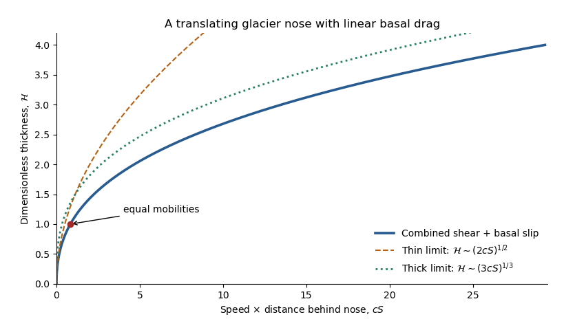
The right side is strictly increasing, giving a unique positive thickness at every $s>0$. With $S=X_N-X$ and $c=d{X}_N/d\tau$, the same relation reads $cS={\mathcal{H}}^3/3+{\mathcal{H}}^2/2$. Its limiting profiles areThe square-root tip reflects basal sliding; the cube-root thicker region reflects internal viscous deformation. Even during the early thick regime, the very nose is thin and has the square-root inner form. At late times that sliding balance governs nearly the whole profile. The dimensionless crossover thickness is $\mathcal{H}=1$ and its distance is $S=5/(6c)$; the early thick cube-root outer profile matches this smaller sliding region. The diverging geometric slope at the idealized tip also marks the local limit of the long-wave shallow-ice approximation.