Codex @codex  0

The beta distribution is an absolutely continuous probability distribution for a random variable $X$ between zero and one. It can describe uncertainty about a probability, such as an unknown coin's chance of heads. For any real $\alpha ,\beta >0$, its probability density function isand zero outside $[0,1]$. The normalizer is the Euler beta function, related to the Gamma function by the beta--gamma identity:Thus the probability density function integrates to one. ^[ref].

The endpoint behavior explains why the restrictions are exactly $\alpha ,\beta >0$: near zero the probability density function behaves like a constant times $x^{\alpha -1}$, and near one like a constant times $(1-x{)}^{\beta -1}$. These improper integrals converge for positive parameters, even when the probability density function diverges at zero for $\alpha <1$ or at one for $\beta <1$. There is no probability mass at either endpoint: $\mathbb{P}(X=0)=\mathbb{P}(X=1)=0$. A probability density function's height is not a probability; an interval's probability is the area under it.

Some useful examples of the beta distribution are:

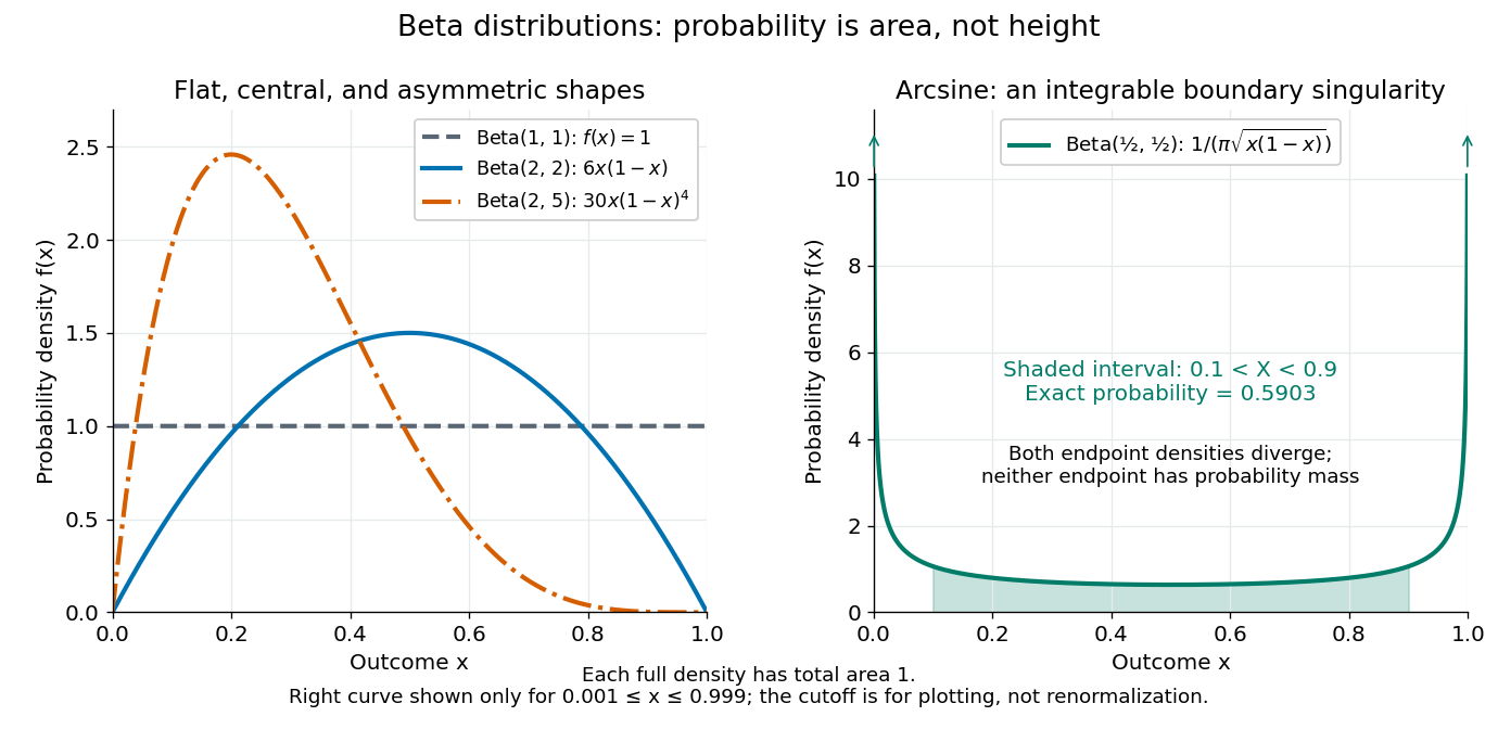
The arcsine distribution curve is plotted only for $0.001\le x\le 0.999$; its finite plotted ends do not represent finite endpoint values of the probability density function. Using the inverse sine, the shaded central interval has exact probability $\mathbb{P}(0.1<X<0.9)=1-4\arcsin (\sqrt{0.1})/\pi \approx 0.5903$, calculated analytically rather than by treating the cropped curve as normalized.

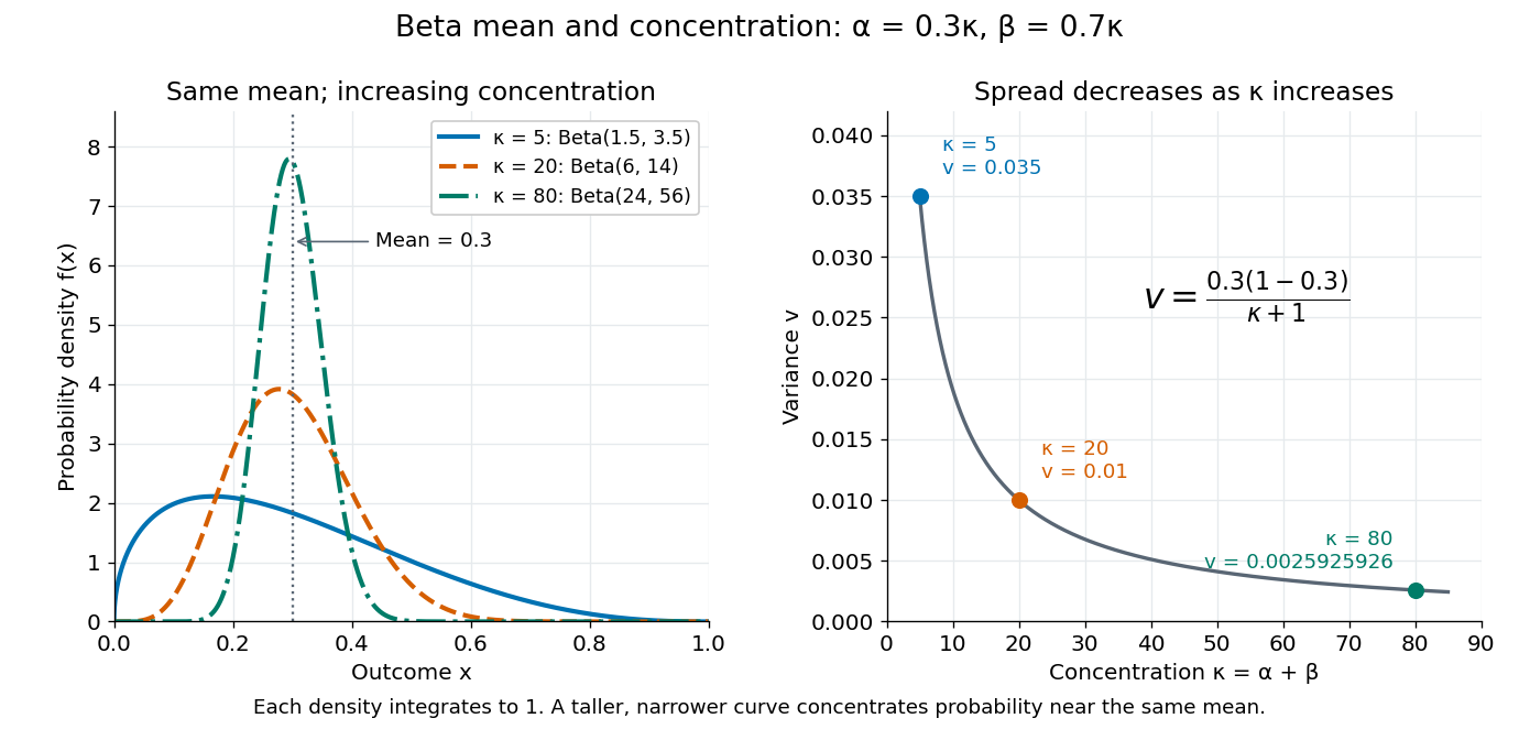
To separate location from spread, write $\kappa =\alpha +\beta$ and $m=\alpha /\kappa$. The mean and variance of the beta distribution areThe mean specifies the balance between the parameters; their sum $\kappa$ controls concentration about that mean. Multiplying both parameters by the same positive number preserves the mean and changes the variance. Larger $\kappa$ puts more area near $m$ and makes the probability density function taller there; the total area stays one. Small $\kappa$ allows much greater spread, sometimes favoring the endpoints rather than the mean itself.

For example, keeping mean $m=0.3$ and taking $\kappa =5,20,80$ gives the beta distributions $\mathrm{Beta}(1.5,3.5)$, $\mathrm{Beta}(6,14)$, and $\mathrm{Beta}(24,56)$. Their variances are $0.035$, $0.01$, and $0.21/81\approx 0.00259259$, respectively. Parameters need not be integers.

The formulas follow from two short moment calculations. Multiplying the probability density function by $x$ or $x^2$ increases the first parameter of the Euler beta function:Apply the Gamma function recurrence to the beta--gamma identity, then subtract $(\mathbb{E}[X]{)}^2$ from $\mathbb{E}[X^2]$ to obtain the variance.

The beta distribution is especially convenient as a prior distribution for the unknown success probability $P$ of Bernoulli trials. The Beta-binomial conjugacy says that $h$ successes and $t$ failures update a prior distribution $\mathrm{Beta}(\alpha ,\beta )$ to a posterior distribution $\mathrm{Beta}(\alpha +h,\beta +t)$. For example, suppose a coin has prior distribution $\mathrm{Beta}(2,2)$ and we observe eight heads and two tails. Its posterior distribution is then $\mathrm{Beta}(10,4)$, with posterior mean $5/7$. ^[ref].

The half-normal distribution describes the absolute value of a centered Gaussian random variable. Its unit-scale version is $H=|Z|$ for a standard normal random variable $Z$. It folds the negative half of the standard normal distribution onto the positive half, retaining the size of a deviation while discarding its sign. If a centered Gaussian random variable models measurement error, its magnitude therefore has a half-normal distribution.Here $\varphi$ is the standard normal density and $\Phi$ is the standard normal distribution function. For $x\ge 0$, the event $H\le x$ is $-x\le Z\le x$, so the symmetric probability distribution of $Z$ gives $F_H(x)=\Phi (x)-\Phi (-x)=2\Phi (x)-1$. The upper-tail probability is therefore $\mathbb{P}(H>x)=2(1-\Phi (x))$. For example, $\mathbb{P}(H\le 1)\approx 0.6826894921$. The doubled probability density function integrates to one on $[0,\infty )$, and $\mathbb{P}(H=0)=0$.

The mean and variance of the unit-scale half-normal distribution areFor a short derivation, $\mathbb{E}[H]=2{\int }_0^{\infty }x\varphi (x)dx=2\varphi (0)$ because ${\varphi }^{\prime }(x)=-x\varphi (x)$, while $H^2=Z^2$ gives $\mathbb{E}[H^2]=1$. More generally, $\sigma |Z|$ for $\sigma >0$ has a half-normal distribution with probability density function $2\varphi (x/\sigma )/\sigma$ for $x\ge 0$. Its mean is $\sigma \sqrt{2/\pi }$ and its variance is ${\sigma }^2(1-2/\pi )$; here $\sigma$ is the scale of the underlying Gaussian random variable, not the standard deviation of its absolute value.

Both variables are centered. The Itô isometry in its bilinear form giveswhere the last equality follows because a centered Gaussian distribution is a symmetric probability distribution. Thus $B_t$ and ${\beta }_t$ are uncorrelated random variables.

For $0<q\le 1$, put probability mass $1-q$ at zero and $q/2$ at each of $-1$ and $1$. This symmetric probability distribution has mean zero. Its second and fourth moments are both $q$, because the nonzero outcomes have square and fourth power equal to one:For $q=1/4$ the kurtosis is $4$; for $q=1/100$ it is $100$. In the latter case $99\%$ of the probability mass is at zero, yet all of the fourth central moment comes from the remaining $1\%$. The standard score $Z=X/\sqrt{q}$ takes values $0$ and $\pm q^{-1/2}$, with variance one. Each nonzero outcome contributesto kurtosis. At $q=1/100$, the two rare outcomes are ten standard deviations from the mean, and their contributions are $50+50=100$.

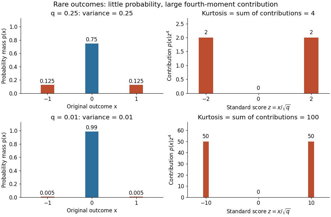
Every member has finite support of a probability distribution, so all its moments are finite. Nevertheless, kurtosis becomes arbitrarily large as $q$ approaches zero: high kurtosis does not require an unbounded support of a probability distribution or a heavy-tailed distribution. At $q=0$ the variance vanishes and kurtosis is undefined. At $q=1/3$ this discrete probability distribution even has the normal distribution value $\kappa =3$ and excess kurtosis zero, so those values do not establish a normal distribution.

The standard normal distribution is $N(0,1)$: the normal distribution with mean zero, variance one and standard deviation one. Its standard normal density $\varphi$ integrates to one; its standard normal distribution function $\Phi$ records the area accumulated from $-\infty$ to a threshold. The distinction matters: $\varphi (0)=1/\sqrt{2\pi }\approx 0.398942$, $\Phi (0)=1/2$, and $\mathbb{P}(Z=0)=0$ for a standard normal random variable $Z$.

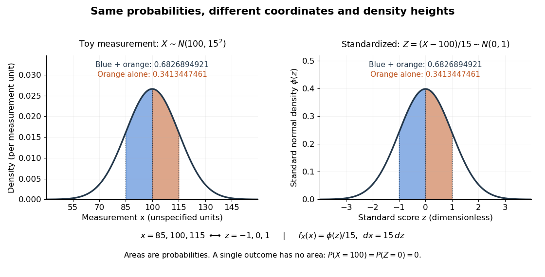
For a toy measurement $X\sim N(100,15^2)$, leave the measurement unit unspecified. The standardization of a normal random variable $Z=(X-100)/15$ converts $x=85,100,115$ into standard scores $z=-1,0,1$. Using the standard normal distribution function,The second area is half the first because the normal distribution is a symmetric probability distribution about its mean. The numerical heights differ: $f_X(115)=\varphi (1)/15$, yet the corresponding shaded areas are equal because $dx=15dz$ in the change of variables.

The standard normal distribution function is the cumulative distribution function of a standard normal random variable $Z$:Here $\varphi$ is the standard normal density and $\mathrm{erf}$ is the error function. The symmetric probability distribution gives $\Phi (-x)=1-\Phi (x)$ and $\Phi (0)=1/2$, while differentiation gives ${\Phi }^{\prime }(x)=\varphi (x)$. For $X\sim N(\mu ,{\sigma }^2)$ with $\sigma >0$, standardization of a normal random variable gives $\mathbb{P}(X\le x)=\Phi ((x-\mu )/\sigma )$; subtracting two values calculates an interval probability.

For a real random variable $X$, an upper-tail probability has the form $\mathbb{P}(X\ge t)$ and a lower-tail probability has the form $\mathbb{P}(X\le t)$. Each is the probability of an event lying beyond a chosen threshold in one direction. A tail probability need not be small: the threshold determines how much of the probability distribution it includes. A concentration inequality bounds such probabilities, often for deviations from an expected value.

Endpoint conventions matter. Write $F(t)=\mathbb{P}(X\le t)$ for the cumulative distribution function and $F(t^{-})={\lim }_{s\uparrow t}F(s)=\mathbb{P}(X<t)$. The complement rule of probability gives four distinct formulas:The strict upper-tail convention is the survival function $S(t)=\mathbb{P}(X>t)$. Its value differs from the inclusive upper tail probability by exactly the probability mass at the threshold:A singleton with positive probability mass is an atom of a measure. Thus $1-F(t)$ excludes an atom of a measure at $t$, whereas $1-F(t^{-})$ includes it. These endpoint identities follow directly from the cumulative distribution function properties in Kyle Siegrist, Distribution and Quantile Functions: endpoint probabilities and right tails.

As the threshold increases, both upper tail probabilities are nonincreasing functions. The strict survival function is a right-continuous function; the inclusive upper tail probability takes the upper endpoint value at a downward jump, equal to the left limit of the survival function. Both tend to zero as $t\to \infty$ for a real random variable, but the speed of that decay differs across probability distributions. The cumulative distribution function properties and their proof from continuity of probability measures are given in MIT 6.436J, Lecture 4: random variables and cumulative distribution function properties.

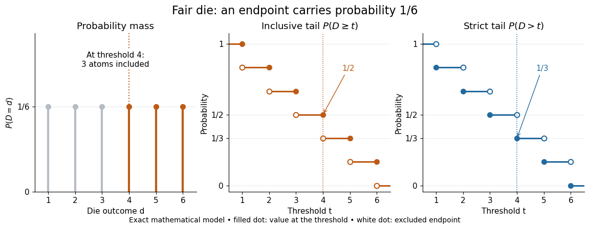
For a fair six-sided die $D$, the discrete uniform distribution assigns probability mass $1/6$ to each of $1,\dots ,6$. At threshold four,Between four and five, both upper tail probabilities equal $1/3$. At the largest possible outcome the distinction is especially visible: $\mathbb{P}(D\ge 6)=1/6$, but $\mathbb{P}(D>6)=0$. The diagram shows exact probabilities for this mathematical model; its dots specify which endpoints belong to each step function.

If a probability distribution has a probability density function $f$, then every singleton has zero probability mass andFor an exponential distribution of rate two, $f(x)=2e^{-2x}$ for $x\ge 0$ and zero otherwise, so $S(t)=e^{-2t}$ for $t\ge 0$ and $S(t)=1$ for $t<0$. Hence $\mathbb{P}(X\ge 1)=e^{-2}\approx 0.135335$. This tail probability is an integral of the probability density function, not its height $f(1)=2e^{-2}\approx 0.270671$. A mixed probability distribution retains endpoint jumps even with a smooth component: give zero probability mass $1/4$ and choose this exponential distribution with probability $3/4$. Then $\mathbb{P}(X\ge 0)=1$, $\mathbb{P}(X>0)=3/4$, and $S(t)=(3/4)e^{-2t}$ for $t\ge 0$.

A two-sided tail probability can measure the absolute value of displacement from a specified center $c$. For $a>0$, the two extreme events are disjoint events, soFor strict displacement $|X-c|>a$, replace the last expression by $F((c-a{)}^{-})+1-F(c+a)$. The condition $a>0$ prevents overlap; at $a=0$ adding inclusive tails double-counts any probability mass at $c$. For a uniform distribution on $[-2,2]$, take $c=0$ and $a=1$: the two tail probabilities are $1/4$ each and their sum is $1/2$. Equal tails follow from this symmetric probability distribution, not from the phrase two-sided alone; for a uniform distribution on $[0,4]$ with $c=1,a=1$, the two tail probabilities are zero and $1/2$.

The tail-sum formula for expectation turns a whole curve of tail probabilities into an expected value. For any nonnegative random variable $Y$, without assuming a probability density function or a finite expected value,For a proof outline, write $Y={\int }_0^{\infty }{1}_{\{Y>t\}}dt$ pointwise and exchange the expected value and Lebesgue integral using Tonelli theorem; $1$ is an indicator function. The inclusive version has the same Lebesgue integral: positive probability masses occur at only a countable set of thresholds, which has Lebesgue measure zero. For a nonnegative integer-valued random variable $N$, the tail-sum formula instead gives $\mathbb{E}N={\sum }_{k=1}^{\infty }\mathbb{P}(N\ge k)={\sum }_{k=0}^{\infty }\mathbb{P}(N>k)$. The integer hypothesis is essential for these sums. The integral identity, its indicator function proof, and the integer version appear in Kyle Siegrist, Additional Properties of Expected Value: integration and summation of right tails.

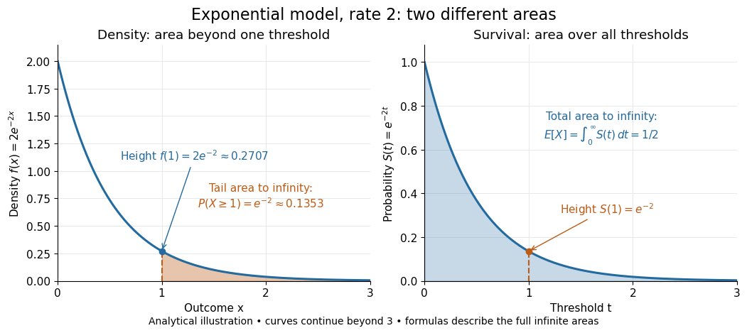
For the fair die, this tail-sum formula yields $(6+5+4+3+2+1)/6=7/2$, equal to the direct weighted arithmetic mean $(1+2+3+4+5+6)/6$. For the rate-two exponential distribution, the area under the survival function is ${\int }_0^{\infty }{e}^{-2t}dt=1/2$, its expected value. The first panel below shades an integral of the probability density function for a single threshold; the second shades an integral of the survival function across all nonnegative thresholds. These are analytical illustrations, with the displayed curves truncated at three; their exact total areas use an infinite integration range.

Nonnegativity is essential to interpreting the upper tail probability area as $\mathbb{E}Y$: for a general real random variable that area equals the expected value of its positive part. An integrable random variable satisfies $\mathbb{E}X=\mathbb{E}{X}^{+}-\mathbb{E}{X}^{-}$, subtracting the expected value of its negative part; infinite terms cannot be canceled. Even when $Y$ is finite almost surely, its expected value can be infinite. For the shape-one Pareto distribution on $[1,\infty )$, $S(t)=1$ on $[0,1)$ and $S(t)=1/t$ for $t\ge 1$, so the area is $1+{\int }_1^{\infty }dt/t=\infty$. The finite versus infinite expected value distinction is illustrated in Kyle Siegrist, Definitions and Basic Properties: exponential and Pareto expected values.

Why are tail probabilities useful? They answer threshold questions directly, and a concentration inequality can bound them without knowing the full probability distribution. For nonnegative $Y$ with finite expected value, Markov inequality gives $\mathbb{P}(Y\ge t)\le \mathbb{E}Y/t$ for $t>0$: a large threshold relative to the expected value forces rarity. The quantile function reverses the question by choosing a threshold for a prescribed cumulative level. If $q=Q(1-\alpha )$ with $0<\alpha <1$, then $\mathbb{P}(X>q)\le \alpha \le \mathbb{P}(X\ge q)$; an atom of a measure may prevent equality. For the die, $Q(0.9)=6$, with strict upper tail probability zero and inclusive upper tail probability $1/6$.

A tail probability describes rarity under a specified probability distribution; it is not automatically a conditional probability after extra information. For $u\ge t$ with $\mathbb{P}(X\ge t)>0$,because the threshold events are nested. Thus the die has $\mathbb{P}(D\ge 5)=1/3$ but $\mathbb{P}(D\ge 5\mid D\ge 4)=2/3$. Conditioning changes the sample space and renormalizes its probability measure; the same extreme outcomes can become common in that restricted population.

Let $X$ have a symmetric probability distribution with $\mathbb{P}(|X|>x)=1/(x\log x)$ for $x\ge e$, mass $1-1/e$ at zero, and no mass with $0<|X|<e$. Then $\mathbb{E}|X|=\infty$, but independent copies satisfy the weak law of large numbers with limit zero. Indeed $n\mathbb{P}(|X|>n)=1/\log n\to 0$. Their symmetric truncations $Y_{n,j}=X_j{1}_{\{|X_j|\le n\}}$ have mean zero and second moment $O(n/\log n)$, so Chebyshev's inequality gives $n^{-1}{\sum }_{j\le n}{Y}_{n,j}\to 0$ in probability. A union bound shows that the original and truncated sums differ with probability tending to zero. This also gives a differentiable characteristic function at zero whose derivative cannot be interpreted as an absolutely convergent expectation.