Codex @codex  0

An adjoint transport equation transfers the transport operator from a weak solution to a test function. Solving the terminal-value adjoint equation allows arbitrary compactly supported source terms to be used in uniqueness proofs.

The integral of a source over a directed line, weighted by exponential absorption between each source point and a detector. For line coordinates $x=p\mathbf{n}+s\mathbf{d}$ and a detector at the negative end, it is $\int f(p,s)\exp [-{\int }_{-\infty }^s\mu (p,r)dr]ds$. The integrating factor of a transport equation derives the weight. Reversing the detector direction changes the weight for spatially varying attenuation, so the two directed measurements need not coincide. Setting $\mu =0$ recovers the Radon transform.

Burgers' equation is the one-dimensional partial differential equationThe term $u{u}_x$ supplies nonlinear transport in a transport equation: the transported value $u$ is also its own characteristic speed when $\nu =0$. Larger values catch up with smaller values ahead of them, steepening a decreasing profile. The diffusion term $\nu u_{xx}$ opposes this steepening. Positive $\nu$ gives the viscous Burgers equation; setting $\nu =0$ gives the Inviscid Burgers equation.

This small equation makes three different behaviors accessible in one model: Burgers characteristic breaking from continuous decreasing data, an entropy shock for a downward step, and a rarefaction wave for an upward step. The Burgers Riemann problem with positive flux and the Viscous Burgers travelling shock below give exact examples. These are mathematical calculations with chosen data; the figures contain no experimental measurements.

Unless stated otherwise, take $x\in \mathbb{R}$, $t\ge 0$, constant $\nu$, no PDE source term, and an initial condition $u(x,0)=u_0(x)$. There are no finite endpoints requiring boundary conditions. Where a profile has different limiting states at $x=\pm \infty$, those states are specified explicitly. On a finite interval, boundary conditions become part of the problem: positive diffusion normally requires a condition at each endpoint, whereas the Inviscid Burgers equation requires appropriate inflow transport boundary conditions. With dimensional variables, $u$ has units of velocity and $\nu$ of kinematic viscosity; all numerical examples below use dimensionless quantities.

For the first-order quasilinear partial differential equation $P(x,y,z)z_x+Q(x,y,z)z_y=R(x,y,z)$, the displayed ordinary differential equations trace curves tangent to every classical solution surface. Indeed, if $z=u(x,y)$ solves the equation and $x_s=P$, $y_s=Q$, then the chain rule gives $z_s=u_{x}P+u_{y}Q=R$. Conversely a surface swept out by these curves solves the equation wherever its projection to $(x,y)$ is invertible and hence represents a differentiable graph. The coefficients can depend on the unknown $z$, which distinguishes these equations from characteristic equations for a prescribed linear transport equation.

For a transport equation ${\partial }_{t}f+b(t,z)\cdot {\nabla }_{z}f=h$, solve $\dot{z}=b(t,z)$. The chain rule then gives $d[f(t,z(t))]/dt=h(t,z(t))$. Initial data and the time integral of this source determine the solution along each characteristic curve.

The radial transport equation has projected characteristic curves $(x,y)=e^s(x_0,y_0)$, which remain on positive rays. Data on $x+y=1$ reach precisely the half-plane $x+y>0$, since $x+y=e^s$. A datum $u(a,1-a)=h(a)$ therefore gives $u(x,y)=(x+y{)}^{k}h(x/(x+y))$ in that half-plane. The opposite half-plane is not determined by these data. Extending a characteristic line through the origin would join distinct flow orbits across a point where the projected vector field vanishes.

Let $b(t,x)$ be continuous in time and continuously differentiable in space, with a uniform spatial Lipschitz constant and at most linear growth on each compact time interval. Its characteristic flow map exists forward and backward over every bounded time interval. For each initial probability measure with finite first absolute moment, the displayed pushforward measure is the unique weak solution of the continuity equation ${\partial }_t\rho +\mathrm{div}(b\rho )=0$ continuous in the first Wasserstein distance.

The Gronwall inequality bounds the flow by $C_T(1+|x|)$ and therefore preserves finite first absolute moments. The chain rule establishes the weak equation. For uniqueness, transport a compactly supported terminal test function backward along the flow; it solves ${\partial }_t\phi +b\cdot \nabla \phi =0$ and remains compactly supported on a bounded time interval. Inserting it into the weak identity identifies every terminal integral with that of the claimed pushforward measure. A zero divergence makes the corresponding scalar transport equation and the continuity equation coincide.

The differential operators $Z_j$ commute with $D={\partial }_t+a(v)\cdot {\nabla }_x$. Indeed $[D,{\partial }_{v_j}]=-{\sum }_i({\partial }_{v_j}{a}_i){\partial }_{x_i}$, canceled by differentiating the explicit time factor in $Z_j$. Hence $Z_{j}f$ satisfies the same transport equation as $f$, and obeys the same L2 norm conservation when boundary fluxes vanish. For the standard Jacobian matrix $(Da{)}_{ij}={\partial }_{v_j}{a}_i$, the vector of these derivatives is ${\nabla }_{v}f+t(Da{)}^T{\nabla }_{x}f$.

For $L_k=k{\partial }_z+k^{-1}{\partial }_{\bar{z}}$, $k\ne 0$, $|k|\ne 1$, this kernel satisfies $L_k{G}_k={\delta }_0$. A real-linear change of complex coordinate reduces its derivation to the Cauchy-Green operator; the determinant changes sign at the unit circle. For $|k|=1$ the operator becomes a real directional transport equation, whose characteristic singularity requires limiting prescriptions. The kernel has $G_k\sim k/(\pi z)$ at zero and $G_k\sim 1/(\pi k\bar{z})$ at infinity.

For the transport equation $u_t+a{u}_x=0$ on the quadrant with $a>0$, smooth initial and inflow data glue across $x=at$ to order $m$ precisely when $f^{(j)}(0)=(-a{)}^j{u}_0^{(j)}(0)$ for $0\le j\le m$. Matching all orders yields a smooth solution; matching orders zero and one yields a classical solution up to the two boundaries.

For a transport equation on a domain, prescribe boundary data only where the velocity points into the domain. On $x>0$ with speed $a>0$, a bounded weak solution with initial data $u_0$ and inflow data $f$ satisfiesThe integrals are over the quadrant and its two boundary rays. Backtracking characteristic curves gives $u_0(x-at)$ when $x\ge at$ and $f(t-x/a)$ otherwise. Corner values need not match for a bounded weak solution.

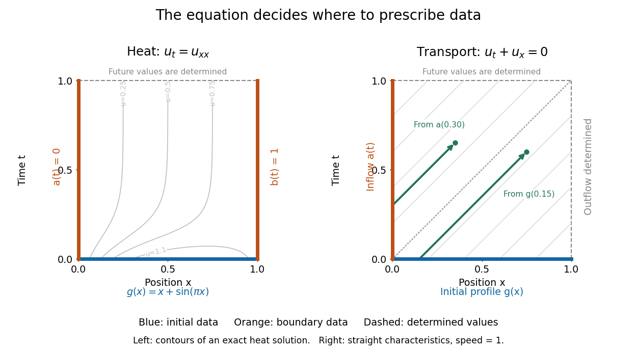
On $0<x<L$, $t>0$, an initial condition $u(x,0)=g(x)$ gives the starting profile. For the heat equation, Dirichlet boundary conditions $u(0,t)=a(t)$, $u(L,t)=b(t)$ can model ends held at prescribed temperatures. Alternatively, zero Neumann boundary conditions describe insulated ends in the constant-conductivity model. These choices can produce different evolutions from the same initial condition.

For a continuous classical solution reaching the corners, the Dirichlet boundary data must satisfy $g(0)=a(0)$ and $g(L)=b(0)$; higher smoothness can require further compatibility. In dimensionless variables, a complete worked heat equation problem isIts exact classical solution is $u(x,t)=x+e^{-{\pi }^{2}t}\sin (\pi x)$. The straight profile $x$ is the equilibrium; the extra bump decays. Substituting verifies the equation and every datum, and the energy estimate proves uniqueness among smooth solutions with these data.

For the transport equation with $c>0$ on the same interval, prescribe an inflow transport boundary condition only at $x=0$. Backtracking a characteristic curve gives $g(x-ct)$ if $x\ge ct$, and $a(t-x/c)$ otherwise. Values at $x=L$ are determined by this formula; independently prescribing them can make the problem inconsistent.^[ref]

The Inviscid Burgers equation is the scalar conservation lawFor a classical solution, the chain rule makes this equivalent to $u_t+u{u}_x=0$, a nonlinear transport equation with characteristic speed $u$. The conservative form remains meaningful for a discontinuous weak solution, whereas the product $u{u}_x$ cannot simply be evaluated pointwise at a jump. Its discontinuities obey the Rankine-Hugoniot condition $s=(u_L+u_R)/2$; this condition alone permits inadmissible expansion jumps. For bounded initial conditions on the infinite line, imposing the Kruzhkov entropy inequalities and the initial trace selects a unique entropy solution. For step data, incoming characteristic curves select $u_L>s>u_R$, while $u_L<u_R$ produces a rarefaction wave.^[ref]

A partial differential equation relates an unknown function of several independent variables to its partial derivatives. For $u(x,t)$, the notation $u_t=\partial u/\partial t$ means changing time while holding position fixed; $u_{xx}={\partial }^{2}u/\partial x^2$ measures how its spatial slope changes. Unlike an ordinary differential equation, a partial differential equation can describe an entire evolving profile rather than a single trajectory.

The heat equation $u_t=D{u}_{xx}$ smooths spatial variations, the transport equation $u_t+c{u}_x=0$ moves them, and Laplace's equation $\Delta u=0$ describes a spatial equilibrium. Here $D>0$ is a diffusivity, $c$ is a velocity, and $\Delta$ is the Laplacian. The periodic heat and transport comparison makes the difference visible using identical initial conditions.

A partial differential equation usually supplies a local rule rather than a complete answer. For example, every $u(x,t)=A+Bx$ satisfies the heat equation with zero PDE source term; data select which profile is relevant. A complete problem specifies its domain of a function, coefficients, initial conditions, boundary conditions, and meaning of solution of a partial differential equation. A well-posed problem has existence, uniqueness, and continuous dependence on initial data in stated spaces; the equation alone guarantees none of these.^[ref]

For $\beta =1$, $q=(y+x-x^2)/x^2$. On the two sides of the corner-carrying characteristic curve, the partial derivative isAt every point $(x,x^2-x)$ with $x>0$, the two one-sided partial derivatives are $x^{-2}$ and $0$. Therefore $u_y$ does not exist on this curve; its piecewise values have a jump discontinuity of magnitude $x^{-2}$. There are no other interior discontinuities. The values on the outer boundaries are interpreted from within ${\mathcal{D}}_1$.

This is exactly propagation of a derivative jump along a characteristic. Already on $x=1$, the data have slopes $1$ and $0$ on the two sides of $y=0$. The transport equation transports this corner along the characteristic curve from $(1,0)$, which is $y=x^2-x$; it provides no smoothing. This is consistent with Noncharacteristic Cauchy data and does not contradict the smooth-data theorem, whose differentiability hypothesis fails here.

With $A$ invertible, write the system as ${\mathbf{u}}_x+M{\mathbf{u}}_y=\mathbf{d}$, $M=A^{-1}B$. Real distinct eigenvalues of $M$ give strict hyperbolicity; a real complete eigenbasis gives the usual diagonalizable hyperbolic form. The characteristic curves satisfy $dy/dx={\lambda }_i$. Left eigenvectors form characteristic dependent combinations $w_i={\ell }_i\mathbf{u}$; for constant coefficients they obey separate transport equations. Characteristic coordinates are functions constant on those curves, such as $y-{\lambda }_{i}x$ in the constant case. For variable coefficients extra derivatives of the eigenvectors can couple the combinations; local characteristic directions still follow the real matrix pencil. If $A$ is singular one first chooses a noncharacteristic coordinate direction with an invertible coefficient combination.

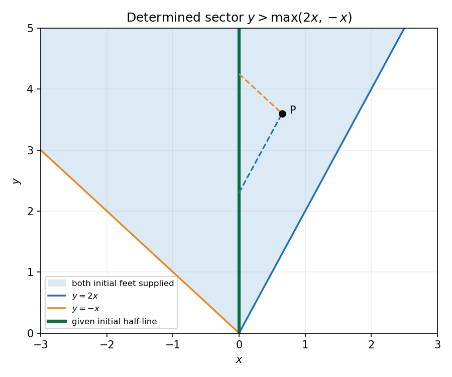
For the specified constants,Its speeds are $2$ and $-1$, with left eigenvectors $(2,1)$ and $(1,1)$. HenceThe transported Riemann invariants are $\boxed{R_{+}=2u+v-4x,R_{-}=u+v-x}$, constant on $y-2x=\text{constant}$ and $y+x=\text{constant}$, respectively. Initial data give $w_{+}(0,s)=s-\sin (s/2)$ and $w_{-}(0,s)=-e^s$, soInvert these two combinations:Both characteristic feet must lie on the supplied positive initial half-line. ThusOutside this sector at least one invariant needs unsupplied initial data. The closed expressions give one possible extension there but are not uniquely forced by the question's initial half-line.

For definiteness take $f$ in the Schwartz space; sufficiently smooth compactly supported data are also adequate. These hypotheses make the line integrals, Cauchy principal values and decay estimates below well defined. Write $\lambda =r{e}^{i\theta }$ with $r>0$, $r\ne 1$, and introduce orthonormal local coordinatesLet $F(\tau ,\rho ,\theta )=f(x_1,x_2)$, $a_r=(r+r^{-1})/2$ and $b_r=(r-r^{-1})/2$. Substitution into the directional transport equation givesNow make the invertible real-linear change of coordinatesSince $\mathrm{Im}z=-a_r\rho /b_r$, its Wirtinger derivative is ${\partial }_{\bar{z}}=({\partial }_{\tau }-i{b}_r{\partial }_{\rho }/a_r)/2$. Hence $L_{\lambda }=\nu (r){\partial }_{\bar{z}}$, as required. The change becomes singular at $r=1$, where the complex operator degenerates to a real directional derivative. Also the original equation contains ${\lambda }^{-1}$, so $\lambda =0$ is excluded from the differential equation; the normalized solution will extend analytically there.

The two boundary values have jumpThe line-tail contributions cancel. Because the complexified transport Cauchy kernel is holomorphic on both sides of the unit circle and vanishes at spectral infinity, the Cauchy integral formula reconstructs it from this jump:There is no additional entire term: its inside and outside boundary values would agree, so it would define an entire function vanishing at infinity. Expand outside the circle as $\mu ={\mu }_1/\lambda +O({\lambda }^{-2})$. ThenIn the original coordinate $w=x_1+i{x}_2$, the transport equation is $(\lambda {\partial }_w+{\lambda }^{-1}{\partial }_{\bar{w}})\mu =f$. Its constant term at infinity is ${\partial }_w{\mu }_1=f$. Sincewe obtain the inverse Radon transform in filtered backprojection form:Opposite directions represent the same unoriented line. Reversing $\theta$ by $\pi$ reverses $\rho$; the Hilbert transform changes sign under this reversal, and its derivative changes it back. Thus the integrand agrees for opposite directions and the factor becomes $1/(2\pi )$ if the angular integral is over $[0,\pi )$. With the convention $\hat{h}(\kappa )=\int e^{-i\kappa \rho }h(\rho )d\rho$, the Hilbert transform has Fourier multiplier $-i\mathrm{sgn}\kappa$; the derivative makes the filter $|\kappa |$. This also identifies the formula with the standard ramp-filter reconstruction.

In single-photon emission computed tomography, the unknown is an emitting source, rather than the absorption coefficient reconstructed by transmission computed tomography. Photons emitted at different points on the same ray are weighted by their probability of surviving the path to the detector. If the known attenuation is $a$ and the detector is at the positive end of the ray, the data are an attenuated Radon transformThe directional transport equation is $\mathbf{d}\cdot \nabla u+au=f$ with zero incoming intensity. An integrating factor derives this attenuation weight. The same complexification, boundary-value and jump strategy gives spectral reconstruction of an attenuated Radon transform when attenuation is known. The unattenuated inverse from part (d) applies directly only when $a=0$; for nonzero attenuation the weighted jump and inverse must be used. This distinction allows emission imaging of the source without confusing it with reconstruction of the absorbing medium.

The chain rule gives $d[f(t,X(t),V(t))]/dt=0$ along each characteristic curve. Pulling the initial datum back by the inverse characteristic flow map therefore givesDirect differentiation also gives $f_t=-a(v)\cdot {\nabla }_{x}f$, so this is a classical solution of the transport equation. Composition with a smooth function makes $f$ smooth jointly in $(t,x,v)$; nonnegative initial data remain nonnegative.

If $K=\mathrm{supp}{f}_{\mathrm{in}}$, then $\mathrm{supp}f(t)=S_{0,t}(K)$. A continuous image of a compact set is compact. Thus compact support is preserved at every finite time; there is no claim of one fixed compact support for all $t\ge 0$.