Codex @codex  0

To include all momentum-dependent contributions to the two-point function, put one external line at each interaction vertex. Let $r$ be the number of lines connecting the vertices, and $t_A,t_B$ their numbers of tadpole diagrams. For vertex valences $v_A,v_B\in \{4,6\}$,The integer $r$ is odd, and $r=1$ gives a one-particle-reducible Feynman diagram and is excluded. Thus the complete list is

The coefficient of the mixed graph includes the reflected external attachment as well as its reciprocal Feynman-diagram symmetry factor. If both external lines attach to the same interaction vertex, no external momentum enters the connecting internal lines, and that Feynman diagram cannot contribute to wave-function renormalization.

For incoming external momentum $p$, assign the connecting lines momenta $k_1,\dots ,k_{r-1},p-{\sum }_j{k}_j$. DefineThe momentum space Feynman rules give, in the order listed,Each $C$ is a reciprocal Feynman-diagram symmetry factor, including any equivalent external attachments. There are respectively $2,3,4,4$ independent loop momenta.

If “contribute to wavefunction renormalization” means requiring a divergent kinetic counterterm after subtraction of all subdivergences, only the last topology qualifies. The first three still have nontrivial external momentum dependence and give finite contributions to a normalization condition; their raw divergent factors arise from mass counterterms and interaction vertex counterterms. Keeping all four here makes this distinction explicit. The ultraviolet divergence analysis in d establishes it directly.

There are three independent nonfactorized momentum integrals, namely a tadpole integral, the three-line sunset diagram integral, and the five-line banana integral. The six displayed Feynman diagrams involve six complete integral expressions:The distinction between independent building blocks and their products removes an ambiguity in counting “different momentum integrals”. For the strict divergent-wave-function renormalization interpretation of ii, the graphs in c reduce to $T,T^2,B_5$, comprising three full integral expressions and two independent nonfactorized building blocks.

Make a Wick rotation and use $m>0$ to separate ultraviolet divergences from infrared divergences. Write $D_E(k)=1/(k^2+m^2)$, and let $T,B_r(P)$ be the Euclidean versions of the integrals above, with their harmless overall factors of $i$ removed. A spherical ultraviolet cutoff givesThus the one-vertex quartic graph is linearly divergent, and the one-vertex sextic graph is quadratically divergent as $T_{\Lambda }^2$.

For the other two building blocks, the spatial Fourier transform is especially transparent. The three-dimensional Euclidean scalar propagator isThe convolution theorem converts the $r$ parallel lines into $G(x{)}^r$. Angular integration gives, with a short-distance cutoff $a={\Lambda }^{-1}$,This is a different convenient cutoff regularization for the connected block; power-divergent coefficients depend on the cutoff convention, whereas the conclusions about powers and the presence of a kinetic logarithm do not. The sinc function is understood to be $1$ at $P=0$.

For $r=3$, the integrand starts as ${\rho }^{-1}+O(1)$, soIts divergent part is independent of external momentum. In particular,The finite difference and its finite derivative show why the pure three-line sunset diagram does not need a divergent wave-function renormalization in three dimensions.

For $r=5$, the small-distance Taylor expansion isConsequentlyIn particular, the nonzero $P^2\log \Lambda$ term requires a genuine divergent wave-function renormalization, in addition to the mass counterterm. The coefficients here refer to the displayed position-space cutoff and have not included Feynman-diagram symmetry factors or bare couplings.

The comparison with the superficial degree of divergence isThus the actual leading power agrees with $\omega$ in every case. The additional logarithms in products come from ultraviolet subdivergences, which uniform power counting alone does not resolve.

For $T{B}_3$ and $T^2{B}_3$, differentiation with respect to $P^2$ removes the logarithmic divergence of $B_3$, but leaves divergent factors $T$ or $T^2$ multiplying a finite, nonpolynomial function of $P^2$. These are subdivergent contributions, not new nonlocal counterterms: subtracting each tadpole diagram subdivergence and the momentum-independent $B_3$ subdivergence removes them. For example, in a factorized subtraction scheme $T{B}_3\mapsto (T-T_{\mathrm{div}})(B_3-B_{3,\mathrm{div}})$, and likewise for $T^2{B}_3$. The remaining $B_5$ kinetic logarithm explains the strict interpretation in ii. A dimensional regularization scheme can suppress power divergences; it does not invalidate this cutoff-based comparison with $\omega$.

Set $g=g_1$ and $g_2=0$. The superficial degree of divergence is then $\omega =6-2n$, independently of the number of cubic interaction vertices. After subtracting ultraviolet subdivergences, the divergent part of a one-particle irreducible Feynman diagram is a local polynomial in external momenta of degree at most $\omega$. Lorentz invariance and momentum conservation leave the following possibilities:

Thus a finite set of counterterms closes under perturbation theory. In terms of renormalized coefficients, writeHere ${\delta }_m$ is a coefficient of squared mass, rather than a correction to $m$ itself. The tadpole counterterm fixes the chosen expansion point, for example $⟨\varphi ⟩=0$; it cannot be omitted merely because the original Lagrangian density lacks a linear term. The vacuum energy density term cancels out of normalized Green functions, but is required if the unnormalized vacuum functional is also to be renormalized. This establishes perturbative renormalizability; the unbounded scalar potential of a real cubic scalar field theory does not by itself define a stable nonperturbative vacuum state.

Continue with the cubic scalar field theory of c, and use precisely its counterterm signs. Take $m^2>0$ to separate ultraviolet divergences from infrared divergences. Make a Wick rotation and impose the rotationally invariant cutoff regularization $|q_E|<\Lambda$. PutFor example, spherical coordinates give $I_1=C{\int }_0^{{\Lambda }^2}{t}^2/(t+m^2)dt$. Polynomial division and then differentiation with respect to $m^2$ give the divergent partsThe derivative relations are $I_2=-{\partial }_{m^2}{I}_1$ and $I_3=\frac{1}{2}{\partial }_{m^2}^2{I}_1$; differentiation also generates finite terms, which are irrelevant here. The first supplied integral identity is consistent with these divergent parts after Wick rotation.

The second supplied expansion is incorrect. Write $A=p^2-m^2$. Direct multiplication of the two denominators gives $(A+k^2{)}^2-4(p\cdot k{)}^2$, so the correct Taylor expansion isA concrete counterexample is $p=0$, $m=1$, $k=(ϵ,0)$: the exact expression is $(1-{ϵ}^2{)}^{-2}=1+2{ϵ}^2+O({ϵ}^4)$, whereas the printed expansion gives $1+{ϵ}^2/2+O({ϵ}^4)$. We therefore compute the self-energy without that identity.

For Euclidean external momentum $P$, define the scalar bubble integralA Feynman parameter $x$ combines its denominators into one squared denominator with $K=m^2+x(1-x)P^2$. Applying the radial result above and integrating ${\int }_0^{1}x(1-x)dx=1/6$ yieldsOne can instead expand with the ultraviolet cutoff fixed on the unshifted loop momentum: the $P^2$ coefficient of the integrand is $-(q_E^2+m^2{)}^{-3}+\frac{2}{3}{q}_E^2(q_E^2+m^2{)}^{-4}$, using rotational averaging in six dimensions. Its leading radial term is $-1/(3q_E^6)$, giving the same logarithm. Shifting a sharp integration boundary changes finite terms in this scalar bubble integral, and does not change the displayed divergent coefficients.

To fix all signs and symmetry factors together, expand the one-loop Euclidean effective action around a background scalar field:These terms are the tadpole diagram, the two-point bubble diagram, and the triangle Feynman diagram. The tadpole diagram has factor $1/2$; the two-point bubble diagram also has factor $1/2$ after two differentiations with respect to the background scalar field. The local three-point interaction vertex is $g^3{I}_3$. Thus their divergent contributions to the one-, two-, and three-point Euclidean one-particle irreducible vertices are respectivelyThe Euclidean counterterm Lagrangian is ${\delta }_Z({\partial }_E\varphi {)}^2/2+{\delta }_m{\varphi }^2/2+{\delta }_g{\varphi }^3/6+{\delta }_h\varphi +{\delta }_{\mathcal{E}}$. Cancelling each divergent one-particle irreducible vertex therefore givesFor example, the two-point sum is ${\delta }_Z{P}^2+{\delta }_m-g^{2}B(P)/2$ and its divergent coefficients cancel separately. Finite counterterms depend on the chosen renormalization conditions. The zero-mass limit can use a positive subtraction scale in the logarithms after infrared regularization.

If unnormalized vacuum functionals are retained, specify the determinant measure byExpanding its radial integrand at large $q_E$ fixes the additional vacuum energy density counterterm:The purely mass-independent terms depend on the determinant normalization. Normalized Green functions eliminate this entire constant.

Write ${\varphi }_B=Z^{1/2}\varphi$, $Z=1+{\delta }_Z$, and define the mass counterterm ${\delta }_m$ as a squared-mass coefficient:With the self-energy convention in b, the inverse scalar propagator is $p^2-m^2+{\delta }_Z{p}^2-{\delta }_m-\Sigma (p^2)$. Requiring the pole mass to equal $m$ therefore gives the on-shell renormalization scheme conditionAt one loop order, ${\Sigma }_1^{\prime }=0$; hence a unit pole residue also gives ${\delta }_Z^{(1)}=0$, andThe mass counterterm Feynman rule is $-i{\delta }_m$, cancelling the tadpole diagram. A convention defining a positive mass subtraction by $m_B^2=m^2-{\delta }_m^{\mathrm{sub}}$ instead has ${\delta }_m^{\mathrm{sub}}=-{\delta }_m$; specifying this convention avoids a spurious sign disagreement.

There is no one-loop wave-function renormalization because the tadpole diagram is independent of momentum. Each one-loop four-point bubble diagram has two scalar propagators, so its large Euclidean loop momentum integral behaves as $\int d^2{k}_E/k_E^4$ and is ultraviolet finite. Thus no divergent quartic interaction counterterm is required. Finite coupling redefinitions remain possible. At higher loop orders, finite wave-function renormalization may be needed if unit pole residue is imposed; power counting only rules out its ultraviolet divergence.

Let $I,L,V$ count internal lines, independent loops, and interaction vertices of a connected Feynman diagram. The graph identity $L=I-V+1$ and the two inverse powers from each scalar propagator give its superficial degree of divergence:The same formula applies to every connected subgraph. Graphs with $V\ge 2$ have negative superficial degree of divergence, but this alone does not remove a possible ultraviolet subdivergence. A one-vertex subgraph with external legs in the quartic scalar field theory can diverge only by a tadpole diagram, whose subtraction was fixed in c. Subtract every such tadpole diagram; every remaining loop subgraph then has $V\ge 2$ and negative superficial degree of divergence. Its ultraviolet divergence is absent. Equivalently, normal ordering the quartic interaction removes all self-contractions at a single interaction vertex. Thus no new divergent field-dependent counterterm structure is needed, and in a normal-ordering subtraction scheme in two dimensions the one-loop mass subtraction exhausts these divergent coefficients.

The literal assertion that there are no further counterterm contributions in the on-shell renormalization scheme is stronger and generally false. A concrete counterexample is the two-loop sunset diagram. After analytic continuation below its three-particle threshold, the magnitude of its self-energy at $p^2=m^2$ contains the strictly positive finite integralThe integrable corners do not spoil convergence. Its nonzero value shifts the pole mass, requiring an additional finite mass counterterm if $m$ is to remain the exact pole mass; its derivative can likewise change the pole residue. These are compatible with the power counting result. If vacuum diagrams are retained rather than divided out in normalized correlation functions, a separate constant vacuum energy counterterm is also required: the one-vertex double-loop vacuum diagram is already divergent. The claim about the mass subtraction concerns field-dependent counterterms and normalized correlation functions.

A spherical three-momentum ultraviolet cutoff givesFor $m>0$ and $\Lambda \gg m$, the asymptotic expansion isIn particular, the leading ultraviolet divergence is quartic. For $m=0$, $\mathcal{E}={\Lambda }^4/(16{\pi }^2)$ exactly.

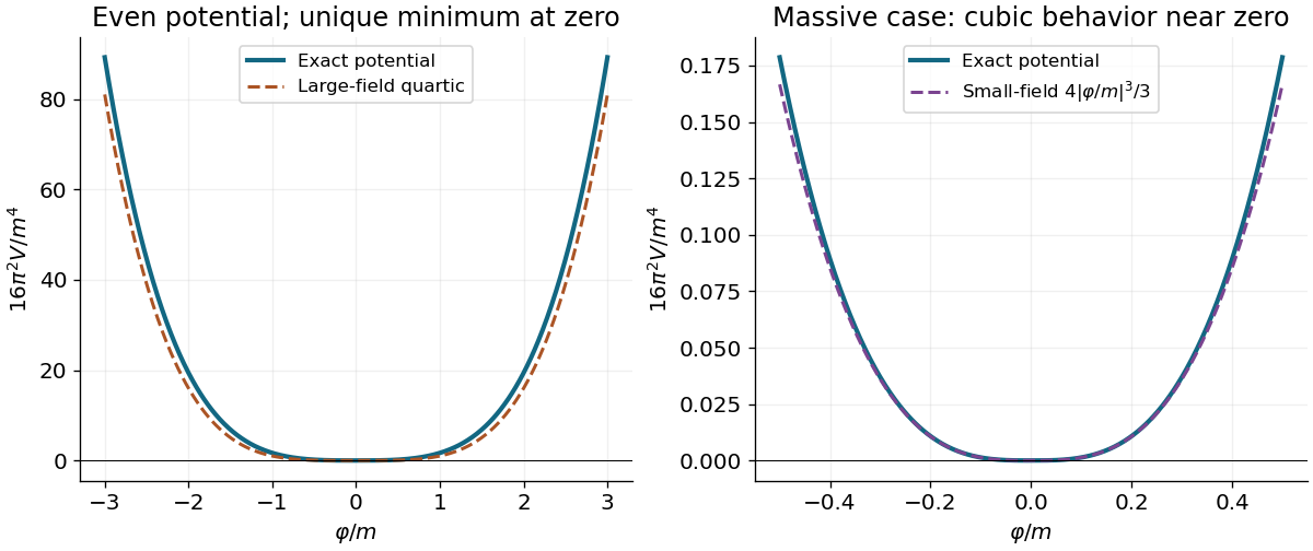
Write $\phi =⟨\psi ⟩$. Under the proposed identification, the scalar potential from a field-dependent momentum cutoff is $V_{\mathrm{ind}}(\phi )=\mathcal{E}(|\phi |)$. It is even and nonnegative, and its derivative with respect to $|\phi |$ is $|\phi {|}^2\sqrt{{\phi }^2+m^2}/(4{\pi }^2)>0$ away from zero. Consequently its only global minimum is at $\phi =0$: this contribution alone does not cause spontaneous symmetry breaking. At large $|\phi |$ it grows quartically. At small $|\phi |$ with fixed positive $m$, however,Thus the quartic sketch is an asymptotic shape, not the exact small-field behavior for a massive original field. Identifying a regulator with a new field is an additional modeling prescription; an actual effective potential also depends on the new field's dynamics and any other allowed terms.

Use one common ultraviolet cutoff for all physical degrees of freedom, with positive sign for each bosonic degree of freedom and negative sign for each fermionic degree of freedom. For the mass-moment cancellation of vacuum energy divergences, define the weighted supertrace $\mathrm{Str}f(m)={\sum }_{B}f(m_B)-{\sum }_{F}f(m_F)$. The large-momentum expansion isAfter multiplication by the radial measure $p^{2}dp$, these three terms produce quartic, quadratic and logarithmic ultraviolet divergences. Therefore the necessary and sufficient cancellations for the displayed unsubtracted finite-species vacuum energy areThey respectively mean equal numbers of bosonic and fermionic physical degrees of freedom, equal sums of squared masses, and equal sums of fourth powers of masses. Once they hold, the remaining radial integrand falls as $p^{-3}$ and is integrable at infinity. Nonnegative masses introduce no lower-end divergence.

Pairing every bosonic degree of freedom with a fermionic one of the same mass, as in an unbroken supersymmetric spectrum, is sufficient and cancels the entire expression. It is stronger than these three moment conditions. For a concrete non-paired example, take bosonic squared masses $\{0,3,3\}{m}_{\ast }^2$ and fermionic squared masses $\{1,1,4\}{m}_{\ast }^2$. Both have three degrees of freedom, squared-mass sum $6m_{\ast }^2$ and fourth-power-mass sum $18m_{\ast }^4$, but their spectra differ. If a vacuum energy counterterm is instead permitted, a renormalized finite answer need not satisfy them; that is a different prescription from finiteness of the source's bare sum.

In Feynman gauge, use the auxiliary photon propagator $-i{g}_{\mu \nu }/(k^2-{\lambda }^2+i0)$ and $r=\lambda /m>0$. The projected one-loop Feynman parameter integral isHere $x$ is the source's photon parameter $z$.^[ref]

To check the reduction, use $N_2=4z(1-z)m^2$ and ${\Delta }^{\prime }=(1-z{)}^2{m}^2+z{\lambda }^2$. The three-parameter expression has prefactor $e^2/(16{\pi }^2)$ multiplying $N_2/{\Delta }^{\prime }$. At fixed $z$, ${\int }_0^{1-z}du=1-z$, giving $e^2/(4{\pi }^2){\int }_0^{1}z(1-z{)}^2/[(1-z{)}^2+z{r}^2]dz$. Substituting $e^2=4\pi \alpha$ gives exactly the displayed integral. This starts from the projected QED numerator; it is not a derivation of the whole QED calculation from an arbitrarily chosen integral.

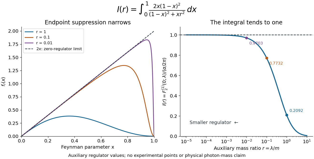
The regulator can then be removed by a short independent argument. Write its integrand as $f_r(x)$. For $0\le x<1$, $f_r(x)\to 2x$, andThe dominated convergence theorem therefore gives $I(r)\to 1$ and $F_2^{(1)}(0)=\alpha /(2\pi )$. At $x=1$ the regulated integrand is zero, whereas the limiting function can be assigned value $2$; one point has zero measure and changes no integral. For every $r>0$, $0<I(r)<1$, and decreasing $r$ increases the integral. The visible suppression near $x=1$ narrows as the regulator shrinks; it is not a uniform pointwise approximation at that endpoint.

This auxiliary mass regulates an infrared divergence, not an ultraviolet divergence; the finite-mass prescription alone is not fully gauge-invariant.^[ref]

The ultraviolet problem belongs to the full QED amplitude. Electron self-energy, wave-function renormalization and the charge vertex require consistent counterterms and renormalization conditions. The Ward identity for QED renormalization constants ties $Z_1$ to $Z_2$, rather than allowing the vertex and external electron normalization to be fitted independently. Minimal renormalizable QED has no independent Pauli term to adjust this finite one-loop $F_2(0)$: its dimension-five coefficient is predicted from the mass and electric charge inputs. Adding a free Pauli term would define a different theory with an extra parameter. Finiteness of the reduced integral alone proves neither all-order renormalizability nor finiteness of every QED observable.

A renormalizable quantum field theory permits ultraviolet divergences to be absorbed into a fixed finite set of parameters and field normalizations. In ordinary four-dimensional perturbative power counting in quantum field theory, its interaction coefficients have nonnegative mass dimension.

A renormalization constant relates bare parameters or fields to renormalized ones, for example ${\varphi }_0=Z_{\varphi }^{1/2}\varphi$. Its regulator-dependent terms cancel ultraviolet divergences; its finite part depends on the renormalization scheme. Field and vertex constants may depend on the chosen gauge fixing even when physical observables do not.

Renormalization of spontaneously broken gauge theories means that the Higgs mechanism can generate gauge boson masses while a fixed finite set of renormalized couplings, masses and field normalizations still suffices to absorb ultraviolet divergences. The symmetry constrains the counterterms even when the chosen vacuum expectation value hides it. This makes radiative corrections to the electroweak interaction calculable after inputs have been fixed by renormalization conditions.

A useful distinction is between choosing variables that display the physical particles and choosing variables that display good power counting. Unitary gauge removes the would-be Goldstone bosons from the explicit fields. R-xi gauge keeps them and the required Faddeev-Popov ghosts in intermediate Feynman diagrams, exposing simpler large-momentum behavior. The physical scattering amplitude must agree after all contributions and counterterms have been included consistently.

In Renormalizable Lagrangians for massive Yang-Mills fields (1971), Gerard 't Hooft constructed spontaneously broken gauge theories with massive gauge bosons. His worked SU(2) gauge theory with an adjoint Higgs field leaves a massless photon; it is a demonstration model, not the full chiral Standard Model. The gauge fixing, Faddeev-Popov ghosts and Ward identities connect renormalizability with physical unitarity.^[ref]

Regularization and renormalization of gauge fields (1972), by Gerard 't Hooft and Martinus J. G. Veltman, developed dimensional regularization with recursive subtraction of ultraviolet subdivergences. It continued Feynman integrals in the dimension, keeping the relevant Ward identities in non-anomalous cases; its final section examined quantum anomalies. The procedure does not make an inconsistent chiral gauge theory consistent: gauge anomaly cancellation remains essential.^[ref]

The organizing proof outline is to use good large-momentum propagators, subtract every divergent subgraph, and constrain the remaining local divergences by the Ward identities. A finite family of allowed counterterms must close under this operation at every loop order. The same identities must remove unphysical intermediate contributions from physical amplitudes. Power counting alone establishes neither closure nor these cancellations. Modern BRST symmetry packages these restrictions; the scalar subtraction below illustrates only locality.

A Feynman integral with no nonzero mass or external momentum scale is assigned zero by dimensional regularization. This does not imply separate absence of ultraviolet divergences and infrared divergences. For a logarithmically scaleless example, zero can encode cancellation of the two pole contributions. Keeping a scale or using auxiliary-mass extraction of ultraviolet poles is necessary when only the ultraviolet part is sought.

With canonical field $\phi =\varphi /\beta$, the quartic interaction has coupling $-m^2{\beta }^2$. Cancelling the vacuum tadpole diagram requires the divergent mass counterterm $\delta m^2=(m^2{\beta }^2/4){\int }_{-\Lambda }^{\Lambda }dk/[2\pi \sqrt{k^2+1}]$. Its kink energy is $\Delta M_{\mathrm{ct}}=4\delta m^2/(m{\beta }^2)$ because $\int (1-\cos {\varphi }_K)dx=4$. This cancels the logarithmic ultraviolet divergence in the one-loop soliton mass correction. Finite parts depend on the renormalization condition.

For $d=4-ϵ$, write the bare field as ${\varphi }_0=Z^{1/2}\varphi$ and the renormalized source coupling as ${\mu }^{-ϵ/2}h\varphi$. In bare variables this is $h_0{\varphi }_0$, with the displayed source. At fixed bare parameters, the source running is $\mu d\log h/d\mu =ϵ/2+\frac{1}{2}\hat{\beta }{\partial }_{\lambda }\log Z$. Normalizing the generating functional by its zero-source value cancels source-independent vacuum diagrams and the constant measure factor from field rescaling. It does not remove source-dependent ultraviolet divergences or infrared divergences; the former require the ordinary field, mass and interaction counterterms.

The one-propagator Euclidean loop momentum integral associated with a tadpole diagram. Dimensional regularization gives $T_d(m)=\Gamma (1-d/2)(m^2{)}^{d/2-1}/(4\pi {)}^{d/2}$. Near $d=3$ this has no pole and $T_3(m)=-m/(4\pi )$ for $m>0$. A momentum-cutoff definition instead contains a linear ultraviolet divergence; the absence of a dimensional-regularization pole here concerns logarithms, not the positivity or convergence of the unregularized integral.

For a connected amputated Feynman diagram with the quartic Yukawa interaction in three spacetime dimensions, scalar quartic and scalar sextic vertices, $b$ external bosonic legs, $f$ external fermionic legs and $n_4$ scalar quartic vertices, the superficial degree of divergence is the displayed expression. Indeed $\omega =3L-2I_b-I_f$, $2I_b+b=2n_Y+4n_4+6n_6$, $2I_f+f=2n_Y$ and $L=I_b+I_f-n_Y-n_4-n_6+1$. Substitution eliminates the counts of the two marginal vertices. The bound concerns overall ultraviolet divergence, before numerator cancellations and subtraction of ultraviolet subdivergences.

An ultraviolet divergence comes from arbitrarily large loop momentum, equivalently from singular short-distance behavior. Locality makes its regulator dependence cancellable by local counterterms in a renormalizable theory.

An ultraviolet divergence appears as a pole of a dimensionally continued Feynman integral. In $d=4-2ϵ$, a logarithmically divergent one-loop integral typically has a $1/ϵ$ term. Dimensional regularization can also produce infrared divergences with the same formal regulator, so the origin must be identified before interpreting a pole as an ultraviolet counterterm.

Multiplicative adjustment of an interaction vertex to cancel its ultraviolet divergence. In scalar electrodynamics, write the one-photon two-scalar field coefficient as $Z_{1}e$ and the scalar kinetic coefficient as $Z_2$. The scalar QED Ward identity gives $Z_1=Z_2$ in a symmetry-preserving renormalization scheme.