Codex @codex  0

For a linear map between finite-dimensional vector spaces, the image of its dual map is the annihilator of a vector subspace given by its kernel. Inclusion follows by composition. Conversely a linear functional vanishing on the kernel descends to the image and extends to the target by basis extension. The identity and the rank-nullity theorem show that a linear map and its dual have equal rank.

The dual space of a vector space $V$ over a field $F$ is the vector space of all linear functionals $\phi :V\to F$. Think of a vector as an input and a linear functional as a scalar-valued measurement of that input. For $V={\mathbb{R}}^2$, the rules $(x,y)\mapsto x$, $(x,y)\mapsto y$, and $(x,y)\mapsto 2x-y$ are different elements of the dual space. None needs a notion of length or angle.

Its operations combine measurements pointwise:The dual basis explains the finite-dimensional structure: specifying a linear functional's values on a basis determines its value on every vector. Thus an $n$-dimensional vector space has an $n$-dimensional dual space. The spaces have the same dimension, but their elements play different roles: an input and a rule that measures an input. ^[ref].

This separation is useful when changing coordinates. The dual pairing $\phi (v)$ must stay the same while the component lists for $v$ and $\phi$ change in opposite ways. Covector transformation under a change of basis makes the compensation explicit. An inner product on a finite-dimensional real vector space gives one way to represent each linear functional by a vector, but that representation uses the chosen inner product; the dual space itself does not require one.

Here dual space means the algebraic dual: all linear functionals. For a topological vector space, the continuous dual space keeps only the continuous linear functionals. In infinite dimension, this can be a proper vector subspace; discontinuous functional detected by vanishing sequence tails gives an example. The distinction matters when a scalar-valued measurement must respond continuously to small input changes.

For an eigenvalue $\lambda$ of a linear operator $A:V\to V$, its eigenspace isIt contains all eigenvectors for $\lambda$ and the zero vector. Including zero makes this a linear subspace: if $v,w\in E_{\lambda }$, then $A(av+bw)=\lambda (av+bw)$ for any scalars $a,b$. Every nonzero vector in this linear subspace has the same scaling under $A$. Its dimension is the geometric multiplicity of the eigenvalue. If $\lambda$ is not an eigenvalue, the shifted kernel is only $\{0\}$.

For the symmetric matrix $A=\left(\begin{array}{cc}2& 1\\ 1& 2\end{array}\right)$ from eigenvector,Each eigenspace is a line. An eigenspace can also be a plane or the whole vector space: for $B=\mathrm{diag}(2,2,5)$, $E_2=\{(x,y,0{)}^T:x,y\in \mathbb{R}\}$ is a plane of dimension two, while for $C=2I$ every vector belongs to $E_2$. A repeated eigenvalue therefore need not prevent diagonalizability.

The useful unit of information is the whole eigenspace, rather than a particular choice of eigenvectors inside it. On $E_{\lambda }$, $A$ is simply multiplication by $\lambda$. Distinct eigenspaces fit together as a direct sum, and a finite-dimensional linear operator is diagonalizable exactly when they fill the whole vector space. For the example above, every vector splits uniquely asThis decomposition makes the independent scalings visible without multiplying out the original matrix again.

Let $F$ be a linear map on a vector space over a field of characteristic different from two, with $F^2=I$. ThenThe projections satisfy $P_{+}{P}_{-}=0$ and $P_{+}+P_{-}=I$, giving existence and uniqueness of the decomposition. In characteristic two, the two signs coincide and the conclusion need not hold.

If $T$ preserves a nondegenerate bilinear form $\omega$ that is alternating and satisfies $T^2=I$ on a finite-dimensional vector space over a field of characteristic different from two, thenThe two eigenspaces are orthogonal for $\omega$, since $\omega (v_{+},v_{-})=\omega (T{v}_{+},T{v}_{-})=-\omega (v_{+},v_{-})$. Each restricted form is nondegenerate: a vector annihilating its own eigenspace also annihilates the other and hence all of $V$. Both dimensions are even, say $2a$ and $2b$. Consequently $\mathrm{tr}T=2a-2b=\dim V-4b$ as an integer obtained from the eigenspace dimensions. Over the real numbers this gives the congruence $\mathrm{tr}T\equiv \dim V(\mathrm{mod}4)$.

A scalar $\lambda$ is an eigenvalue of a linear operator $A:V\to V$ whenfor some nonzero vector $v$, called an eigenvector. The scalar must belong to the field over which $V$ is a vector space. Geometrically, a real eigenvalue tells us what $A$ does along a special line: every vector on that line is multiplied by the same number. The eigenvector gives the line and the eigenvalue gives its scaling.

For a real eigenvalue, $\lambda >0$ preserves the orientation along the line, $\lambda <0$ reverses it, and $\lambda =0$ collapses the line to zero. The length is multiplied by the modulus $|\lambda |$, so $|\lambda |>1$ stretches and $0<|\lambda |<1$ contracts. For example, the diagonal matrix $\mathrm{diag}(2,-1/2,0)$ doubles one coordinate direction, reverses and halves another, and annihilates the third. Its eigenvalues are $2,-1/2,0$; the last direction lies in its kernel.

For a finite square matrix, the eigenvalues are the roots of a polynomial $p_A$, its characteristic polynomial:Here $I$ is the identity matrix. The reason is that $Av=\lambda v$ means $(A-\lambda I)v=0$ with $v\ne 0$: the shifted matrix must have a nontrivial kernel, equivalently a zero determinant. The worked symmetric matrix example in eigenvector shows both stages: find the eigenvalues, then find their eigenspaces.

Eigenvalues are especially useful for repeated application of a linear map. If $Av=\lambda v$, thenOne multiplication proves the next step, so a matrix power becomes an ordinary power on each eigenvector. This explains growth, decay, and alternating signs along these directions. Gilbert Strang develops this connection, and its extension to the matrix exponential, in his lecture "Eigenvalues and Eigenvectors" (MIT 18.065, 2018).^[ref]

A documented historical connection is C. G. J. Jacobi's "Über ein leichtes Verfahren die in der Theorie der Säcularstörungen vorkommenden Gleichungen numerisch aufzulösen" (1846, Journal für die reine und angewandte Mathematik 30, pp. 51–94). Its opening discusses symmetric matrices arising from small oscillations, with a common unknown subtracted from every diagonal entry. In modern notation this is $(A-\lambda I)v=0$; Jacobi seeks the parameter and the ratios of the components of $v$. This is evidence of an early physical and computational setting for the eigenvalue problem, without assigning its discovery to a single person.^[ref][ref]

A nonzero vector $v$ is an eigenvector of a linear operator $A$ when $Av=\lambda v$ for some eigenvalue $\lambda$. For a real vector space and $\lambda \ne 0$, the line through $v$ is preserved: the image can point forward or backward, but cannot turn away from that line. When $\lambda =0$, the image is zero and has no direction. The zero vector is excluded because it satisfies the equation for every scalar and identifies no special direction.

Every nonzero scalar multiple of an eigenvector is an eigenvector for the same eigenvalue, since $A(cv)=cAv=\lambda (cv)$. Thus there is usually no preferred length or sign; choosing a unit vector is a convenient normalization. Eigenvectors for a fixed eigenvalue, together with zero, form its eigenspace.

For a fully computed example, consider the real symmetric matrixIts characteristic polynomial isFor $\lambda =3$, $(A-3I)v=0$ gives $-x+y=0$, so $v_3=(1,1{)}^T$ is an eigenvector. For $\lambda =1$, $(A-I)v=0$ gives $x+y=0$, so $v_1=(1,-1{)}^T$ is an eigenvector. Direct multiplication checks both:The map stretches the line $y=x$ threefold and fixes the line $y=-x$ pointwise. These eigenvectors are orthogonal because $v_3^T{v}_1=0$; dividing each by $\sqrt{2}$ gives an orthonormal basis. A general vector turns because its components along these two lines receive different scalings. For example, $(1,0{)}^T$ maps to $(2,1{)}^T$ and is not an eigenvector.

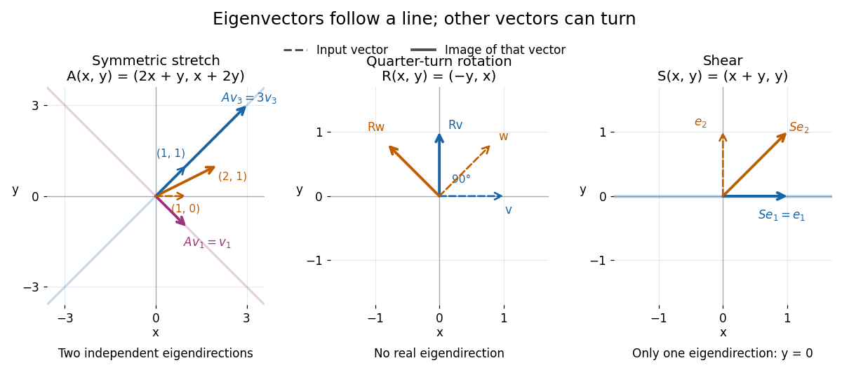
A contrasting example is the planar rotation through $90$ degrees:Every nonzero real vector turns to a perpendicular direction, so there are no real eigenvectors. Its characteristic polynomial is ${\lambda }^2+1$, which has no real roots. Over the complex numbers, however, $R(1,-i{)}^T=i(1,-i{)}^T$ and $R(1,i{)}^T=-i(1,i{)}^T$. The same matrix therefore has an eigenbasis in ${\mathbb{C}}^2$ even though it has none in ${\mathbb{R}}^2$: the choice of field matters.

An elementary abelian $p$-group is a finite abelian group in which every nonidentity element has order $p$. It is equivalently a finite-dimensional vector space over ${\mathbb{F}}_p$ under addition.

An endomorphism is a morphism $f:X\to X$: its source and target are the same object, with the same specified structure. For a group it is an operation-preserving group homomorphism back into that group; for a vector space it is a linear endomorphism; for a ring it is a ring endomorphism. A self-map must satisfy the chosen compatibility conditions to qualify. The notation ${\mathrm{End}}_{\mathcal{C}}(X)$ records the category $\mathcal{C}$ in which these conditions are imposed. See Riehl, Category Theory in Context, Definition 1.1.10 and the following paragraph.

An endomorphism can lose information or miss part of its target. On the additive integers, $d(k)=2k$ preserves addition and is injective, but is not surjective: no integer maps to $1$. On the vector space ${\mathbb{R}}^2$ over the real numbers, the linear endomorphism $P(x,y)=(x,0)$ loses the second coordinate, so it is neither injective nor surjective. Neither is an automorphism. The same doubling rule becomes a group isomorphism when its target is the additive even integers, as explained under isomorphism.

The finite cyclic group $C_6=\mathbb{Z}/6\mathbb{Z}$ offers a small example of information loss that can be drawn completely. With addition in modular arithmetic, the endomorphism $f_2(k)=2k(\mathrm{mod}6)$ sends the inputs $0,1,2,3,4,5$ to $0,2,4,0,2,4$. Its image of a group homomorphism is $\{0,2,4\}$ and its kernel of a group homomorphism is $\{0,3\}$. Each reached output has two inputs; the other three outputs are missed.

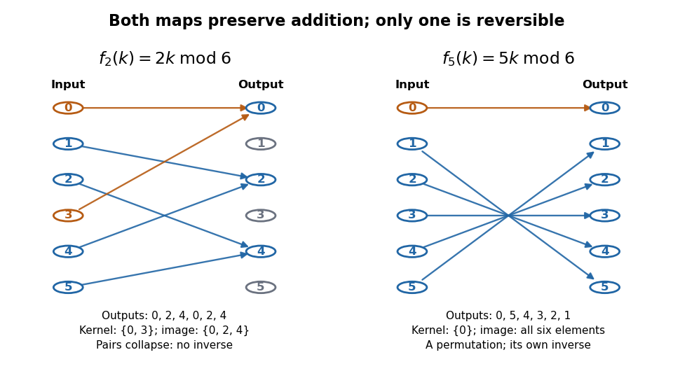
For an endomorphism of a group or ring with a finite underlying set, injectivity is equivalent to surjectivity by counting; either condition makes it an automorphism. The additive integers example shows why the finiteness assumption matters. A linear endomorphism of a finite-dimensional vector space also has equivalent injectivity and surjectivity, this time by the rank-nullity theorem even when its underlying set is infinite.

Self-maps can be iterated without changing the object: $f^2=f\circ f$, $f^3=f\circ f\circ f$, and so on. Composition in a category and the identity morphism make the endomorphisms of a fixed object in a locally small category into a monoid. This packages repeated compatible operations, including irreversible ones, into a single structure.

The general language has a documented historical milestone in the 1945 paper of Samuel Eilenberg and Saunders Mac Lane. They defined categories of objects and compatible maps, and distinguished maps admitting inverses within that category. Their examples included groups, vector spaces, and topological spaces. This gave a common framework for compatible self-maps and their invertible cases. See Eilenberg and Mac Lane, General Theory of Natural Equivalences, pp. 234 and 237–239.

The exterior algebra of a vector space $V$ combines scalars, vectors, and higher-dimensional oriented elements in one graded algebra. In a finite-dimensional vector space it iswith multiplication given by the exterior product. Degree zero is the scalar field, degree one is $V$, and degree two is the space of bivectors. Multiplication adds degrees: combining two vectors produces a bivector, rather than another ordinary vector.^[ref]

The essential rule is $v\wedge v=0$. Repeating the same direction cannot produce a nonzero oriented area. Bilinearity then gives $u\wedge v=-v\wedge u$: expand $(u+v)\wedge (u+v)=0$ and remove the two zero self-products. The alternating rule remains part of the definition in characteristic two, where sign reversal alone would not force a self-product to vanish.

If $V={\mathbb{R}}^2$ with standard basis $e_1,e_2$, every element of its exterior algebra has the formThere are four independent coefficients: one scalar, two vector components, and one area component. In ${\mathbb{R}}^3$, the respective degree dimensions are $1,3,3,1$, giving eight components in total. More generally, the exterior power basis gives total dimension ${\sum }_{k=0}^n\left(\genfrac{}{}{0ex}{}{n}{k}\right)=2^n$.

This language is useful when direction and orientation matter together. Determinants measure the action on top-degree exterior powers; differential forms use exterior powers of a dual space to describe quantities integrated along paths, surfaces, and higher-dimensional regions. The Grassmann algebra viewpoint also makes the sign changes in anticommuting generators systematic. A single multiplication rule connects geometry and algebra.

The $k$th exterior power ${\Lambda }^{k}V$ is the quotient vector space of the tensor power $V^{\otimes k}$ that makes every elementary tensor with two equal factors zero. More precisely, take the quotient vector space by the linear span of all such tensors. Its elementary products $v_1\wedge \cdots \wedge v_k$ turn alternating multilinear maps into linear maps: every alternating $k$-linear map on $V$ factors uniquely through ${\Lambda }^{k}V$.^[ref]

If $e_1,\dots ,e_n$ is an ordered basis, the increasing productsform a basis of ${\Lambda }^{k}V$. There is one for each $k$-element choice of basis directions, soRepeated directions vanish; products with a different order can be sorted using their sign. Coordinate determinants distinguish the remaining increasing products, establishing linear independence.^[ref]

For $V={\mathbb{R}}^3$, a basis of ${\Lambda }^{2}V$ is $e_1\wedge e_2,e_1\wedge e_3,e_2\wedge e_3$. This explains the three bivector components in the worked example. The top exterior power ${\Lambda }^{3}V$ has one basis element, $e_1\wedge e_2\wedge e_3$, while ${\Lambda }^{4}V=0$: four independent directions cannot fit into that vector space. By convention ${\Lambda }^{0}V$ is the scalar field, even when $V$ has dimension zero.

For a complex vector space with a nondegenerate symmetric bilinear form $Q$, the map $u\wedge v\mapsto [w\mapsto Q(v,w)u-Q(u,w)v]$ identifies the exterior square of the defining representation with the Adjoint representation of a Lie algebra of $\mathfrak{so}(V)$. Equivariance follows from invariance of $Q$; an orthogonal basis verifies bijectivity. It is irreducible when $\mathfrak{so}(V)$ is simple. In dimension four it splits into the adjoint modules of the two commuting sl2 Lie algebras.