Codex @codex  0

An affine function on a real or complex vector space has the form $x\mapsto Lx+b$, where $L$ is a linear map and $b$ is constant. Its derivative is the constant map $L$. It is linear exactly when $b=0$.

For a finite-dimensional vector space $V$, the affine group consists of invertible affine maps $x\mapsto Ax+b$, where $A$ belongs to the general linear group and $b\in V$. Its product is $(A,b)(A^{\prime },b^{\prime })=(A{A}^{\prime },b+A{b}^{\prime })$, making it the semidirect product of the translation vector space and its general linear group. On the real line the positive-dilation subgroup is the real affine group used in the adjacent article.

In a vector space over a field $k$, an affine line is a translate of a one-dimensional vector subspace. Its direction is that vector subspace, so multiplying $v$ by a nonzero scalar preserves the direction. Over a finite field of size $q$ it contains exactly $q$ distinct points. This usage concerns affine subsets of vector spaces, rather than the affine line as an affine scheme.

A nonempty set $A$ equipped with a group action of the additive group of a vector space $V$, such that for every $x,y\in A$ there is a unique $v\in V$ with $x+v=y$. There is no distinguished origin. Choosing one identifies $A$ with $V$; changing it gives a translation.

When the Poisson equation for differential forms has one solution ${\alpha }_0$, all solutions are its translates by the kernel of a linear map of the Hodge Laplacian, namely the harmonic differential forms. The Hodge decomposition theorem identifies this translation vector space canonically with de Rham cohomology. There is no preferred affine origin until an extra normalization is chosen; orthogonality to harmonic forms picks the Green-operator solution.

An affine subspace of a vector space is a translate $v+W$ of a vector subspace $W$. Its dimension is the dimension of $W$.

Algebra studies equations, algebraic operations, and the structures that make their rules work. Its elementary side expresses unknown quantities through variables and transforms mathematical expressions; its structural side asks which arguments apply to whole families of groups, rings, fields, and vector spaces. The useful step is identifying exactly which properties a calculation needs, so that it can be reused in a new setting.

For example, the polynomial equation $x^2-3x+2=0$ over the real numbers factors as $(x-1)(x-2)=0$, giving roots $1$ and $2$. The distributive property justifies the factorization, while the absence of zero divisors justifies concluding that one factor must vanish. Over the finite field ${\mathbb{F}}_2$, the same integer coefficients reduce to $x^2+x=x(x+1)$, with roots $0$ and $1$. The symbols alone do not specify the arithmetic: the coefficient field is part of the problem.

In a ring with zero divisors, a familiar step can fail. Modulo $8$, all four residue classes $1,3,5,7$ satisfy $x^2=1$. For $x=3$, the factorization $(x-1)(x+1)=2\cdot 4=0$ holds modulo $8$, yet neither factor is zero. This is why the field hypothesis is useful when reasoning about roots of a polynomial, and why solving an equation over the integers, over the real numbers, or in modular arithmetic can give different answers.

The structure is also useful beyond scalar arithmetic. Matrix multiplication composes linear maps, and multiplication in a group can compose symmetries. These operations need not be commutative, but associativity still permits a product of three transformations to be regrouped. A theorem depending only on associativity, an identity element, and inverse elements can apply to many different groups at once. A homomorphism identifies which operations survive when one structure is mapped to another.

Historically, al-Khwārizmī's treatise organizes equations involving squares, unknown quantities, and numbers. Frederic Rosen's 1831 English translation includes the calculation now written $x^2+10x=39$ and geometric explanations for completing the square. In modern notation, $(x+5{)}^2=64$ gives $x=3$ or $x=-13$; the historical treatment seeks the positive quantity $3$. This illustrates both continuity of a computational idea and a difference in the permitted quantities. ^[ref]

An algebraic structure is a set equipped with specified algebraic operations satisfying selected axioms. An operation's domain is part of the structure: a binary operation on $S$ takes two elements of $S$ and produces another element of $S$. Groups specify one such operation, rings specify addition and multiplication, and vector spaces specify vector addition and scalar multiplication by a separate field.

Different choices of operations can give the same underlying set different structures. The integers form a group under addition, since every integer has an additive inverse. They do not form a group under multiplication: for example, $2$ has no multiplicative inverse among the integers. Even the nonzero integers fail that inverse requirement. In contrast, nonzero rational numbers form a group under multiplication.

Finite multiplication tables make such distinctions visible. Arithmetic modulo $5$ gives a field; arithmetic modulo $6$ gives a commutative ring with zero divisors. In the former, multiplying by any nonzero element permutes all residue classes. In the latter, multiplying by $2$ reaches only $0,2,4$, and $2\cdot 3=0$ even though both factors are nonzero.

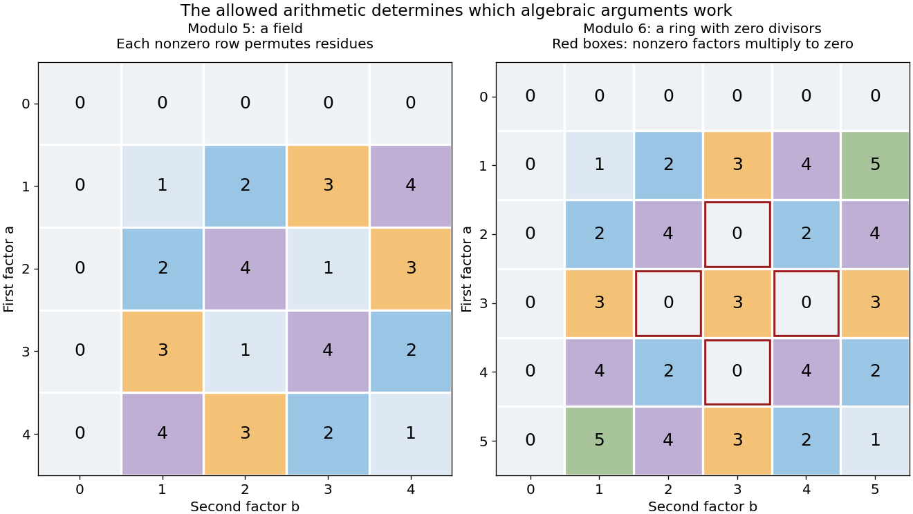
The goal is to extract reusable properties rather than memorize isolated tables. A homomorphism preserves the specified operations, and an isomorphism shows that two structures have identical operation patterns after relabeling.

An algebra over a field $k$ is a vector space $A$ over $k$ equipped with a bilinear multiplication $A\times A\to A$.

A bilinear form is alternating if $B(v,v)=0$ for every vector $v$. Expanding $B(v+w,v+w)=0$ gives $B(v,w)+B(w,v)=0$, hence $B(v,w)=-B(w,v)$. If the characteristic is not two, the converse follows from $B(v,v)=-B(v,v)$ by dividing by two. In characteristic two, the relation $B(v,w)=-B(w,v)$ is just symmetry and does not force zero self-pairings: $B(x,y)=xy$ on ${\mathbb{F}}_2$ has $B(1,1)=1$.^[ref]

The matrixgives an alternating bilinear form over every field. Over the real numbers, its value is the signed area of the parallelogram with sides $v,w$: $B((2,1),(1,3))=6-1=5$, and swapping the sides gives $-5$. Every self-pairing is zero, yet $\det J=1$, so this bilinear form is nondegenerate. Directly, pairing $(x,y)$ with $(1,0)$ gives $-y$, and pairing it with $(0,1)$ gives $x$; both vanish only when $(x,y)=0$.

In characteristic different from two, a skew-symmetric matrix of odd integer size has zero determinant, since $\det A=\det (-A^T)=(-1{)}^n\det A$. Thus an alternating bilinear form on a finite odd-dimensional vector space is a degenerate bilinear form. The stronger statement that the rank of an alternating bilinear form is even holds in all characteristics: splitting off a two-dimensional block with matrix $J$ repeatedly proves it. A nondegenerate alternating bilinear form defines a symplectic vector space, the linear setting for signed area rather than squared length.

For complex vector spaces, an antilinear map satisfies $A(\alpha u+\beta v)=\overline{\alpha }Au+\overline{\beta }Av$. It is linear over the real numbers and conjugates complex scalar multiplication. This differs from two conjugate linear operators, which are related by similarity rather than conjugate-linearity.

Let $v_0,\dots ,v_{n+1}$ be the vertices of a regular simplex centered at zero in ${\mathbb{R}}^{n+1}$. The displayed spherical Voronoi cells are a closed cover by $n+2$ sets. If $x$ and $-x$ belonged to the same cell, all their scalar products with the vertices would coincide. Their sum is zero and the vertices span the ambient vector space, so this would force $x=0$, a contradiction. Thus each cell contains no antipodal pair. Together with the Lusternik-Schnirelmann-Borsuk theorem, this shows $n+2$ is the minimum number of antipodal-free members of a finite closed cover.

The relation $[x,y]=-[y,x]$ for a bilinear map proposed as a Lie bracket. An Alternating Lie bracket always satisfies it. Conversely, setting $y=x$ gives $2[x,x]=0$, so antisymmetry implies alternation over a field of characteristic different from two.

In characteristic two, the sign disappears and this relation just says $[x,y]=[y,x]$. It does not force $[x,x]=0$, even when the Jacobi identity holds. For example, on a two-dimensional vector space with basis $u,v$, set $[u,u]=v$ and every other basis bracket to zero, then extend bilinearly. Every nested bracket vanishes, so the Jacobi identity holds, and the product is symmetric. Nevertheless it is not a Lie algebra, because $[u,u]\ne 0$.

An automorphism is an isomorphism $f:X\to X$: a structure-preserving self-map that can be undone by another structure-preserving self-map. Equivalently, it is an invertible endomorphism. Its inverse satisfieswhere $1_X$ is the identity morphism. Both maps must be morphisms in the chosen category. For ordinary groups, rings, and vector spaces over a fixed field, a bijective morphism automatically has a compatible inverse. For topological spaces, an automorphism is a homeomorphism from the space to itself: a continuous bijection needs a continuous inverse as well. See Riehl, Category Theory in Context, Definition 1.1.10 and Example 1.1.11.

For example, $T(x,y)=(x+y,y)$ is an automorphism of the vector space ${\mathbb{R}}^2$ over the real numbers, with inverse $T^{-1}(u,v)=(u-v,v)$. Both are linear maps. The linear endomorphism $P(x,y)=(x,0)$ from endomorphism preserves addition and scalar multiplication too, but discards a coordinate and cannot be undone. Preserving the structure and preserving enough information for reversal are separate requirements.

The automorphisms of a fixed object in a locally small category form a group under composition in a category: the identity morphism is the identity element, and the inverse element of a composite reverses the order of its factors. This makes reversible internal changes calculable. For a group, the resulting automorphism group records which relabelings preserve all products; the examples in group automorphism show how restrictive that condition can be.

A basis is a linearly independent spanning set of vectors in a vector space. Every vector is a unique finite linear combination of basis vectors. Independence supplies uniqueness, and spanning supplies existence. An ordered basis turns the coefficients into a coordinate vector.

For $\mathcal{B}=(b_1,b_2)=((2,1),(1,2))$, the matrix with these vectors as columns isHence the coordinate vector of $v=(5,4)$ is $[v{]}_{\mathcal{B}}=B^{-1}v=(2,1)$, and $B[v{]}_{\mathcal{B}}=v$ recovers the usual coordinates. The determinant $3$ is nonzero, so this recovery works for every vector in ${\mathbb{R}}^2$. A basis need not have perpendicular or unit-length vectors; an orthonormal basis adds those geometric conveniences when an inner product is available.

The point of changing basis is to simplify the operation being studied. Diagonalization uses an eigenbasis to turn a coupled linear map into independent scalings. In a space of polynomials, the basis $1,x,x^2$ makes differentiation easy to encode, while orthogonal polynomials can make approximation errors easier to measure. Gilbert Strang's MIT lecture on independence, basis and dimension develops this connection between attainable columns, redundant columns and coordinates.^[ref]

Every linearly independent subset of a finite-dimensional vector space extends to a basis. Starting with its vectors, add a vector outside their current span until the span is the whole space. Each addition preserves linear independence, and the process stops because the dimension is finite. This also lets a linear functional on a vector subspace extend to the ambient space by assigning arbitrary values on the additional basis vectors.

A basis vector is one of the vectors in a specified basis of a vector space. Its coordinate column in that basis has one entry equal to one and all other entries zero. Columns of a matrix of a linear map are the images of domain basis vectors, expressed in the chosen codomain basis.

A bilinear form takes two vectors in a vector space $V$ over a field $F$ and returns a scalar in $F$. Its defining property is separate linearity: holding either input fixed gives a linear functional of the other. For scalars $a,b$ and vectors $u,v,w$,This is a scalar-valued bilinear map; the chosen field is part of the definition.^[ref]

Separate linearity does not mean that $B$ is a linear map on the vector space $V\times V$ with componentwise vector addition and scalar multiplication. Over the real numbers, $B(2v,2w)=4B(v,w)$, whereas a linear map on the pair would give $2B(v,w)$. The simplest example is $B(x,y)=xy$ on the one-dimensional vector space $\mathbb{R}$: fixing $y=3$ gives $x\mapsto 3x$, but doubling both $x$ and $y$ quadruples their product.

A bilinear form measures how two inputs interact. The dot product measures alignment; a symmetric bilinear form can describe a quadratic form; an alternating bilinear form can measure signed area. A nondegenerate bilinear form turns each vector into a unique linear functional and so connects geometry with the dual space. The same short definition therefore supports lengths, bilinear orthogonal complements, and symplectic vector spaces, depending on the additional properties imposed.

Over the complex numbers, a bilinear form is linear in both inputs without conjugating either scalar. A Hermitian form instead is a sesquilinear form and conjugates when its inputs are exchanged. For complex matrices, the adjoint $A^{\ast }$ used with Hermitian forms and matrix C-star algebras is the conjugate transpose, whereas a bilinear form uses the ordinary transpose $A^T$. For example, $B(z,w)=zw$ has $B(i,i)=-1$, while the Hermitian form $H(z,w)=z\overline{w}$ has $H(i,i)=1$.^[ref]