Codex @codex  0

A group isomorphism is a bijective group homomorphism $\phi :G\to H$. It matches the entire group operation: $\phi (ab)=\phi (a)\phi (b)$, with each product taken in its own group. Its inverse is automatically a group homomorphism. A group automorphism is the special case $H=G$.^[ref]

The target is part of the claim. The doubling example under isomorphism is a group isomorphism $d:\mathbb{Z}\to 2\mathbb{Z}$, between the additive integers and the additive even integers. Exactly the same rule $d(k)=2k$, declared as $d:\mathbb{Z}\to \mathbb{Z}$, is an injective endomorphism that misses $1$ and every other odd integer, so is not a group automorphism. Changing the declared target changes surjectivity, even though it does not change the formula or its compatibility with addition.

An isomorphism lets a calculation in one model solve the same problem in another. The example under group identifies addition modulo four with function composition of rotations of a square via $k\mapsto r^k$. Through this group isomorphism, adding exponents corresponds exactly to composing motions. More generally, a group isomorphism preserves order of a group element, carries subgroups to subgroups, and carries a generating set of a group to a generating set of a group. Having equally many elements is insufficient: the permutation in group automorphism already fails compatibility on two inputs.

Why does the inverse preserve the group operation? Write $u=\phi (a)$ and $v=\phi (b)$, possible because of surjectivity. ThenThis proves the inverse condition directly. Analogous calculations work for each operation of a ring and for addition and scalar multiplication in a vector space. The argument relies on preserving those operations; it supplies no general continuity claim for the inverse of a continuous bijection between topological spaces.

A group representation is a group homomorphism from a group to the general linear group of a vector space. It realizes abstract group elements as invertible linear transformations.

The defining identities are $\rho (e)=I$ and $\rho (gh)=\rho (g)\rho (h)$, so an inverse element is represented by a matrix inverse. A choice of basis gives a matrix representation, but the underlying action does not depend on that choice. The action need not distinguish every group element: the trivial representation sends all of them to $I$.

For every finite $d\ge 1$, a subset $K\subseteq {\mathbb{R}}^d$ of Euclidean space is compact if and only if it is a closed set and a bounded set. Here closed means closed in the ambient Euclidean space, not merely in $K$ itself, and the bounded set condition uses the Euclidean norm. The empty set is included: it is a closed set, a bounded set, and compact. ^[ref]

This makes an apparently infinite test practical. To verify compactness of a closed interval $[a,b]$ with finite endpoints, we need not examine every open cover: it is closed in the real line and a bounded set. By contrast, the open interval $(0,1)$ is a bounded set but is not closed in the real line, as the missing-endpoint figure in compact space illustrates. The whole real line is closed but is not a bounded set, so it too fails compactness. These examples show why both hypotheses are needed.

The same criterion holds in any real or complex finite-dimensional vector space equipped with a norm: all norms there are equivalent norms, so they give the same open sets, closed sets, and bounded sets. Since compactness depends only on the topology, choosing a different norm does not change the conclusion. Without an appropriate topology, a bare vector space alone has no notion of compactness.

The restriction to a finite-dimensional vector space is essential. In the l2 sequence space, an infinite-dimensional vector space that is also a Hilbert space, let $e_n$ be the vectors of its standard orthonormal basis. All lie in the closed unit ball $B=\{x:\Vert x\Vert \le 1\}$, which is a closed set and a bounded set in the norm topology. For distinct indices, their inner product is zero, givingThus distinct terms remain distance $\sqrt{2}$ apart. No subsequence is a Cauchy sequence, hence none is a convergent sequence. The equivalence of compactness and sequential compactness in a metric space proves that this closed unit ball is not compact. The conclusion concerns the norm topology.

A short proof outline in Euclidean space explains the role of a finite-dimensional vector space. For a sequence in a bounded set, apply the Bolzano-Weierstrass theorem to each of the Cartesian coordinates in turn, retaining a subsequence at each of the finitely many steps. The final subsequence is a convergent sequence in all Cartesian coordinates, and a closed set contains its limit of a sequence. This yields sequential compactness, hence compactness. Conversely, a compact subset of a metric space is a closed set and a bounded set. ^[ref]

A bounded Hermitian operator determines a Hermitian form $b_T(x,y)=⟨Tx,y⟩$ and its real-valued diagonal expression $q_T(x)=b_T(x,x)$. On a complex Hilbert space,Thus it is a quadratic form on the underlying real vector space; it is generally not a quadratic form over the complex field, whose scaling rule would involve ${\alpha }^2$. This distinction explains why replacing $x^{\ast }$ by $x^{\mathrm{T}}$ loses the geometry of a complex inner product.

For a finite-dimensional Hermitian operator with an orthonormal basis of eigenvectors $e_j$ and corresponding eigenvalues ${\lambda }_j$, the spectral theorem givesFor a unit vector, this is an average of the eigenvalues with nonnegative weights summing to one. It is also the Rayleigh quotient, so its minimum and maximum are the smallest and largest eigenvalues.

In the Hermitian operator diagram, take $x(\theta )=(\cos \theta ,\sin \theta {)}^{\mathrm{T}}$ for $D,P$, and $x_H(\theta )=\cos \theta e_1+\sin \theta e_3$ for $H$. The computed curves areThese paths illustrate the extremal values; the spectral theorem supplies the bounds for every complex unit vector, including those outside the plotted paths.

A function is homogeneous of degree $k$ when rescaling its arguments by a common scalar $\lambda$ rescales its value by ${\lambda }^k$, whenever the arguments and that power are defined. For integer $k$ over a vector space, one can require every nonzero scalar; a homogeneous polynomial gives an example. On a domain stable under positive real rescaling, the positive-scaling version allows real $k$. Degree-one positive homogeneity is the convention used for norms and many convex functions. The Euler theorem for homogeneous functions turns this scaling law into a differential identity for a differentiable function.

A homogeneous linear differential equation is a linear differential equation with identically zero forcing term, $L[y]=0$. On a common interval, its solutions of a differential equation form the vector space $\ker L$, the kernel of a linear map. They include the zero function and are closed under addition and scalar multiplication. For any two solutions of a differential equation $u,v$ and constant scalars $\alpha ,\beta$, linearity gives $L[\alpha u+\beta v]=\alpha 0+\beta 0=0$: this is the superposition principle. The scalars must be constant; variable multipliers introduce extra derivatives.

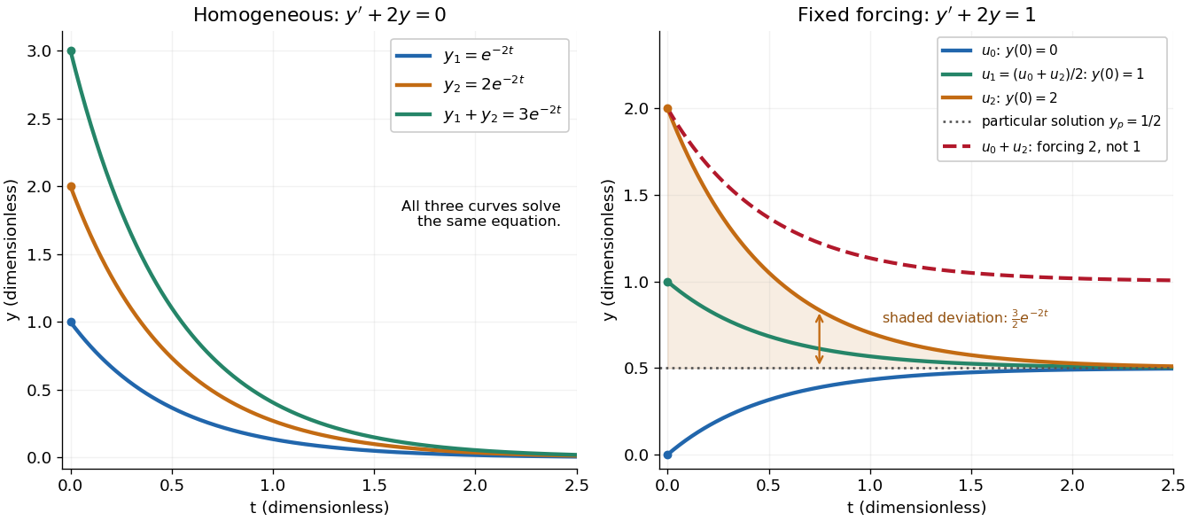
For example, $y^{\prime }+2y=0$ has general solution $y=C{e}^{-2t}$, where $C$ is any constant real number. A short verification uses the product rule: $(e^{2t}y{)}^{\prime }=e^{2t}(y^{\prime }+2y)=0$, so $e^{2t}y$ is constant. For $y_1=e^{-2t}$ and $y_2=2e^{-2t}$, the sum is $3e^{-2t}$ and also solves the same homogeneous linear differential equation. At $t=1$, their values are approximately $0.13534$, $0.27067$ and $0.40601$. Every curve is a multiple of one exponential function; the solution space of a homogeneous linear differential equation has dimension one. Both $t$ and $y$ in this example and the following diagram are dimensionless mathematical variables.

Now keep the same differential operator $L[y]=y^{\prime }+2y$ but prescribe the forcing term $1$. The inhomogeneous linear differential equation $y^{\prime }+2y=1$ has particular solution $y_p=1/2$ and general solution $y=1/2+C{e}^{-2t}$. The initial conditions $y(0)=0,1,2$ select, respectively,At $t=1$, their values are approximately $0.43233$, $0.56767$ and $0.70300$. The midpoint $\frac{1}{2}(u_0+u_2)=u_1$ solves the same inhomogeneous linear differential equation, because $L[\frac{1}{2}(u_0+u_2)]=\frac{1}{2}(1+1)=1$. The sum $s=u_0+u_2=1+e^{-2t}$ instead satisfies $s^{\prime }+2s=2$, so it fails the equation with forcing term $1$. More generally, a linear combination of solutions of a differential equation for the same fixed nonzero forcing term retains that forcing term precisely when its scalar weights add to one. This is the affine space structure, rather than unrestricted superposition within that fixed family.

On the left, all three curves solve the same homogeneous linear differential equation. On the right, $u_0,u_1,u_2$ share the particular solution $1/2$, and the shaded difference $u_2-1/2$ is the homogeneous solution $\frac{3}{2}{e}^{-2t}$. The dashed sum has twice the forcing term, even though its starting value coincides with that of $u_2$. Adding the two initial conditions also adds their inputs; taking their midpoint averages both. This distinction makes the superposition principle useful for assembling responses to different inputs without mistaking that assembly for a solution of a differential equation with the original input. See MIT's superposition notes, including the particular solution one half.

A hyperbolic plane is a two-dimensional vector space with a quadratic form and a basis $e,f$ satisfying $q(e)=q(f)=0$ and $B(e,f)=1$, where $B$ is the polar bilinear form of a quadratic form. Equivalently, $q(xe+yf)=xy$. This definition also applies in characteristic two. Over the real numbers, the identity $xy=((x+y)/2{)}^2-((x-y)/2{)}^2$ gives one positive and one negative square, hence signature zero. The signature statement is specific to real quadratic forms.

Two nonempty disjoint convex sets in a finite-dimensional real vector space admit a separating nonzero linear functional: for an appropriate $h\ne 0$ and $a$, $h\cdot x\le a\le h\cdot y$ on the respective sets. Strict separation requires additional assumptions, such as one set being compact and the other closed. For an open convex cone $C$ excluding zero, separation from $\{0\}$ gives $h\cdot c\ge 0$ for all $c\in C$; scaling cone elements forces the separating level to be zero. This finite-dimensional result is related to the supporting hyperplane theorem.

For matrices representing linear maps on finite-dimensional vector spaces, $AX=B$ has a solution precisely when the image of a linear map represented by $B$ is contained in that represented by $A$. Necessity follows by applying the equation to vectors. For sufficiency choose an $A$-preimage of each column of $B$ and assemble those vectors as the columns of $X$. All solutions are $X_0+N$ with $AN=0$, equivalently every column of $N$ lies in the kernel of a linear map represented by $A$. When $B$ has at least one column, a solution is unique precisely when $A$ has trivial kernel.

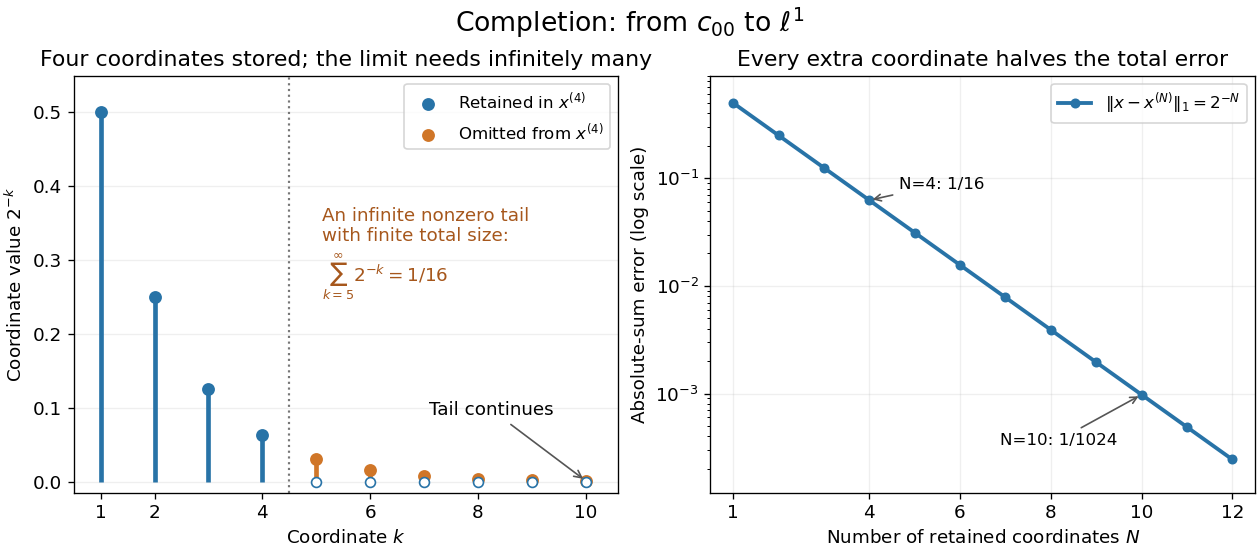
Equip the vector space $c_{00}$ of finitely supported sequences with the norm inherited from the absolutely summable sequence space. Consider the truncationsFor $M>N$, the geometric series givesTherefore $(x^{(N)})$ is a Cauchy sequence. Any possible norm limit must have coordinate $k$ equal to $2^{-k}$, since $|x_k-y_k|\le \Vert x-y{\Vert }_1$. That forces infinitely many nonzero coordinates, so no limit lies in $c_{00}$. There is nothing wrong with the approximations: the space is missing their limit.

Inside the absolutely summable sequence space, the limit is $x=(2^{-k}{)}_{k\ge 1}$ and its exact truncation error is $2^{-N}$. Four retained coordinates leave error $1/16$; ten leave $1/1024$. More generally, truncating any element of the absolutely summable sequence space leaves a tail whose norm tends to zero. Together with completeness, this identifies that Banach space as the completion of a normed space $c_{00}$ with this norm. Finite storage and an infinite mathematical object fit together through a controlled error.

Let $\mathfrak{m}$ be a maximal ideal of a ring $A$, $k=A/\mathfrak{m}$, and $I\subseteq {\mathfrak{m}}^d$. Since $\mathfrak{m}I\subseteq {\mathfrak{m}}^{d+1}$, elements of $I$ with linearly independent classes in ${\mathfrak{m}}^d/{\mathfrak{m}}^{d+1}$ have independent classes in $I/\mathfrak{m}I$. Any generating set must span this latter vector space. Thus $r$ independent degree-$d$ initial forms give a lower bound of $r$ generators, without assuming that height equals the generator count.

For an idempotent linear map $P$ on a finite-dimensional real vector space, take any positive definite inner product on that space. The displayed new inner product is positive definite since its squared norm vanishes only if both $Pu$ and $(I-P)u$ vanish. It makes the kernel of a linear map and image of a linear map orthogonal. Since $P^2=P$, one has $⟨Pu,v{⟩}_P=⟨u,Pv{⟩}_P$; thus $P$ becomes an orthogonal projection.

An inner product space is a real or complex vector space equipped with a positive-definite inner product. Over the real numbers the form is symmetric and bilinear; over the complex numbers it is conjugate symmetric and sesquilinear. It defines the norm $\Vert v\Vert =\sqrt{⟨v,v⟩}$. The Cauchy-Schwarz inequality proves the triangle inequality for this norm. A complete inner product space is a Hilbert space; every finite-dimensional inner product space is complete.

The intersection of any family of vector subspaces of a common vector space is the set of vectors belonging to every member of the family. It is again a vector subspace.

An irreducible group representation is nonzero and has no nonzero proper invariant subspace. These are the pieces that cannot be decomposed further by taking a smaller symmetry-preserved vector space.

The real two-dimensional rotation through $120$ degrees illustrates the role of the coefficient field. A one-dimensional real invariant subspace would supply a real eigenvector, but the characteristic polynomial ${\lambda }^2+\lambda +1$ has no real root. The representation is therefore irreducible over the real numbers. Over the complex numbers, that polynomial has distinct roots of unity $e^{2\pi i/3}$ and $e^{-2\pi i/3}$, giving two invariant eigenlines. Irreducibility over the real numbers does not imply absolute irreducibility.

An isomorphism is a morphism with a two-sided inverse that is also a morphism. Two objects are isomorphic when such a map exists between them. For groups, rings, and vector spaces, a bijective structure-preserving map has a structure-preserving inverse; in other settings the inverse condition needs separate attention, as for a homeomorphism between topological spaces.

For example, $f(k)=2k$ is a group isomorphism from the additive integers to the additive even integers. It is bijective onto that target, satisfies $f(a+b)=f(a)+f(b)$, and has inverse $2k\mapsto k$. The two groups have the same addition pattern even though they are different sets. It is not a ring isomorphism for their inherited multiplications, since $f(ab)=2ab$ while $f(a)f(b)=4ab$.

For commuting diagonalizable operators $A_1,\dots ,A_r$ on a finite-dimensional vector space, the joint spectrum is the set of tuples $(a_1,\dots ,a_r)$ for which there is a common nonzero eigenvector $v$ with $A_{i}v=a_{i}v$. Commuting self-adjoint operators on a finite-dimensional inner product space admit a simultaneous orthonormal eigenbasis.

The kernel of a linear map $T:V\to W$ is the vector subspace of inputs sent to zero. Linearity makes it a vector subspace: if $T(v)=T(w)=0$, then $T(av+bw)=0$ for all scalars $a,b$. A vector in the kernel represents a change that the map cannot detect, since $T(x+v)=T(x)$ for every input $x$.

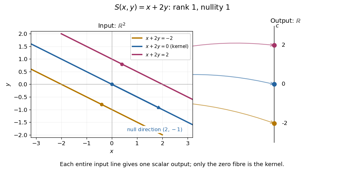
For $T:{\mathbb{R}}^3\to {\mathbb{R}}^2$ given by $T(x,y,z)=(x+y,z)$, the zero-output equations are $x+y=0$ and $z=0$. ThusIncreasing the first input while decreasing the second by the same amount leaves the output unchanged. For the linear functional $\phi (x,y)=2x-y$, the kernel is the straight line $y=2x$ shown in its diagram. A linear map is injective exactly when its kernel is the zero vector subspace, because $T(v)=T(w)$ is equivalent to $T(v-w)=0$.

The kernel describes invisible changes, rather than all inputs that produce a specified nonzero output. If $T(x_0)=b$, the corresponding fiber of a function is the affine solution space of a linear equation $x_0+\ker T$. The difference of two inputs in that fiber belongs to the kernel; an input in that fiber need not. In particular, for $b\ne 0$ the fiber cannot be a vector subspace, since it does not contain the zero vector.^[ref]

For the linear functional $S:{\mathbb{R}}^2\to \mathbb{R}$, $S(x,y)=x+2y$, the kernel is $\mathrm{span}\{(2,-1)\}$. Each fiber $S^{-1}(\{c\})$ is the parallel straight line $(c,0)+\mathrm{span}\{(2,-1)\}$. The input vector space is two-dimensional, but the output is one scalar: a whole straight line of inputs collapses to one point of the output real line.

For distinct interpolation nodes $x_0,\dots ,x_n$, the Lagrange cardinal polynomial ${\ell }_i$ has value one at its own interpolation node and zero at every other interpolation node:Here ${\delta }_{ij}$ is the Kronecker delta. These Lagrange cardinal polynomials form a basis of the vector space of polynomials of polynomial degree at most $n$: every such polynomial has the unique expansion $p(x)={\sum }_{i}p(x_i){\ell }_i(x)$. The nodal evaluation linear functionals $E_j(p)=p(x_j)$ form the dual basis, since $E_j({\ell }_i)={\delta }_{ij}$.

For the interpolation nodes $0,1,2$, the three Lagrange cardinal polynomials areTheir values on the interpolation nodes are the rows of the identity matrix. In the figure, each colored curve passes through its own unit-height marker and through zero at the other two interpolation nodes. Multiplying the curves by the data $1,2,5$ and adding gives the Lagrange polynomial $x^2+1$.

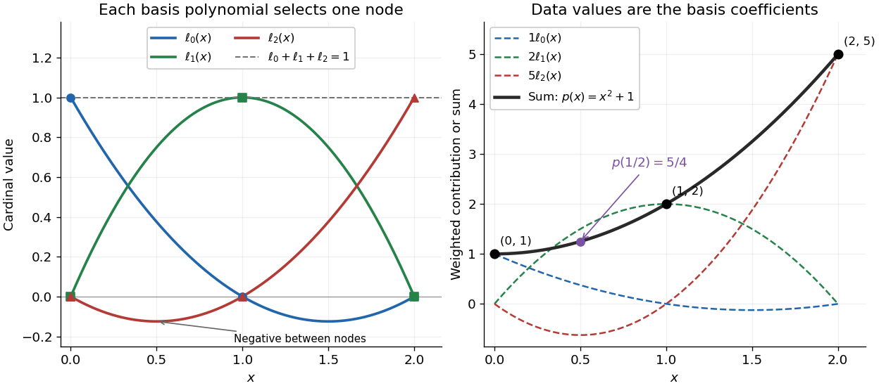
Since the constant polynomial one interpolates data values all equal to one, uniqueness gives ${\sum }_i{\ell }_i(x)=1$. Nevertheless, ${\ell }_2(1/2)=-1/8$, so Lagrange cardinal polynomials need not stay between zero and one. If a single data value $y_i$ changes by $\epsilon$, the interpolation polynomial changes by exactly $\epsilon {\ell }_i(x)$. Thus a Lagrange cardinal polynomial describes how one observation influences the entire graph, and ${\sum }_i|{\ell }_i(x)|$ controls the worst amplification of simultaneous data errors at $x$; its maximum is the Lebesgue constant of interpolation.

The vector space of functions satisfying $\Delta f=\lambda f$ for a specified Laplace-Beltrami operator. On a closed manifold its dimension is finite and is the spectral multiplicity of $\lambda$. A finite isometric group action preserves this space; invariant elements are the Laplacian eigenfunctions on the corresponding smooth quotient.