Phase space combines all independent canonical coordinates and momenta. Its Hamiltonian velocity has divergence by equality of mixed derivatives. Thus an infinitesimal material phase volume has zero fractional rate of change. This is Liouville's theorem, valid also for explicitly time-dependent Hamiltonians. It preserves fine-grained volume, not necessarily the area of any projected coordinate pair.
Define the plasma parameter as the number in a Debye sphere, ; some conventions omit . A good classical plasma has many particles in a screening volume, , and a system size much larger than , so collective fields dominate individual encounters.
A collision here means cumulative Coulomb deflection that significantly changes a particle's velocity, not necessarily a literal hard-sphere impact. A collisionless description requires the phenomenon's timescale to be short compared with the appropriate collision time, and its length scale short compared with the mean free path. Parametrically up to convention-dependent constants, with Coulomb logarithm representing the range of impact parameters. Many oscillations can then occur before collisional relaxation. The formula itself presupposes the weak-coupling regime.
Rapid longitudinal oscillations in a weakly collisional plasma compress the velocity distribution primarily along one direction. There is insufficient time for collisions to redistribute that energy among three directions; the effective one-dimensional adiabatic exponent is . Ordinary monatomic-gas sound with local collisional equilibrium has three translational degrees of freedom, giving . Thus belongs to the stated kinetic/time-scale limit, not to every thermodynamic process involving ionized gas.
As , the scattered kernel is ; as , it is . Therefore on the left and on the right, with
Equal asymptotic wavenumbers give , . Squaring the first amplitude proves the requested expression. These are current ratios, which would require a velocity factor if the two asymptotic potentials differed.
Circular edge-on motion gives and center-of-mass balance gives . Eliminate using the preceding period relation:
Thus when . For a non-edge-on orbit the measured velocity instead determines to this accuracy; neglecting eccentricity is also part of the stipulated model.
A coordinate transformation considered solely as a relabeling of events has no independent observable outcome: changing labels changes neither a detector record nor a clock comparison. But the Lorentz transformations also express substantive relations between operationally realized inertial coordinates. With clocks and rulers specified, their velocity-dependent time dilation, length relations and velocity composition make testable claims about how material systems and electromagnetic signals behave.
The distinction matters for synchronization. One-way coordinate light speed depends on how distant clocks are synchronized; a conventional alteration changes the displayed transformation law while leaving two-way timing observations unchanged. It would therefore be incorrect to regard every coefficient in an unspecified coordinate formula as a separately measurable physical fact. Testable content comes from the transformation together with the protocol and dynamical behavior of the systems implementing the coordinates.
Tests can compare clock proper times, decay lifetimes or resonance behavior across relative motion and orientation. Agreement supports Lorentz-invariant kinematics and the associated matter dynamics over the range tested; it does not prove exact invariance at every possible scale. A rival theory with an undetectable preferred frame can reproduce the same observations by changing its explanatory commitments. Empirical equivalence of that rival does not make the observable clock relations untestable.
Thus the answer is qualified: transformations as passive mathematical changes are not experiments, while Lorentzian relations among specified measuring procedures have substantial empirical consequences. Separating these roles avoids both treating coordinate convention as a measured force and declaring the entire relativistic structure immune to evidence.
Homogeneity makes the inertial transformation linear. Align origins at , let the second origin have velocity , and impose isotropy and reciprocity. Then , , . If the same limiting signal speed has trajectories in both systems, substituting these two trajectories fixes . Requiring the inverse to have the same form with fixes . Continuity at rest selects the positive square root:
Light enters this derivation through the empirical/in-principle operational identification of the invariant speed and Einstein synchronization. Group, homogeneity and isotropy arguments can instead derive a family with a universal parameter , and . They do not by themselves determine whether or a positive finite value. Empirical light propagation or other relativistic dynamics identifies for our world. Consequently a derivation need not assume light as its first premise, but it must acquire the physical invariant-speed structure somewhere rather than extract it from linearity alone.[ref]
Bohmian mechanics retains definite particle positions and deterministic trajectories, which makes it resemble classical mechanics at one level. But the guiding dynamics depends on a wavefunction obeying the Schrödinger equation, with velocity schematically . For many particles this wavefunction is defined on configuration space and can be entangled. The velocity of one particle can consequently depend on the configuration of distant particles. Classical-looking trajectories therefore do not entail classical locality or separability.
Writing also yields a Hamilton-Jacobi-like equation with quantum potential . The quantum potential is not generally a sum of ordinary pair potentials in three-space; its configuration dependence carries the nonclassical correlations. A stationary real bound-state wavefunction can give a stationary particle configuration, unlike the orbit one might infer from a classical Coulomb picture. Measurement outcomes are contextual: the actual apparatus interaction helps determine which position record is produced.
With the quantum-equilibrium distribution , the guidance and wave equations preserve that distribution and reproduce the usual quantum statistics. Determinism alone does not establish that distribution; equilibrium or typicality is an additional explanatory component. The theory also leaves philosophical choices about whether the wavefunction is a physical field, a law-like object or part of a broader ontology.
The significant departure is therefore not simply replacing chance by hidden classical motion. It is the entangled guiding structure, nonlocal dependence and contextual relation between measurements and properties. The retained particles make the account continuous with some classical intuitions, while its actual law and ontology depart substantially from classical many-body mechanics.[ref][ref]
In cylindrical coordinates the orthogonal velocity components are , , . Their squared magnitudes add, and . Thus . Taking the curl gives , consistent with the prescribed field.
Velocity differentiation gives . The coordinates and are cyclic, so are conserved. The radial momentum generally changes. In particular the conserved axial canonical momentum differs from the axial mechanical momentum by .
Use rotating basis vectors with , . The inertial velocity is . The two fixed rotating anchors are , so the spring lengths are . Combining kinetic and elastic energies gives
A constant elastic offset has no dynamical effect.
Hamilton's equations define phase-space velocity . Its divergence is
Thus infinitesimal phase-space volumes are preserved, assuming sufficient differentiability. This is Liouville's theorem; spatial density alone need not be incompressible because the statement concerns the combined coordinate-momentum space.
The plasma parameter is the mean number of electrons in a Debye sphere. With electron Debye length ,
Large describes weakly coupled collective screening; a single electron does not dominate its screening cloud. For a small uniform electron displacement relative to fixed ions, the restoring field gives , hence
This cold-electron oscillation estimate neglects thermal dispersion and ion motion.
Using the stipulated collision-time approximation,
With and , the kinetic estimate gives
The elementary single-speed estimate corresponds to ; velocity averaging and the stated collision model are represented by the supplied . A detailed Coulomb transport calculation also contains a Coulomb logarithm and cannot be inferred precisely from this simplified expression.
The electron thermal energy density is . Transporting all of it at the thermal speed gives the free-streaming scale
For heat flowing in the positive direction, . Inserting into gives
This flux-limiting criterion expresses the failure of a local diffusive description when an electron samples a substantial change in temperature over a transport path.
For the stipulated carbon plasma and , setting the gradient equal to gives a critical flux fraction of order . Fourier transport is invalid according to this test when ; a still larger actual gradient raises the critical value. Thus the source's request for a minimum has the inequality reversed: the calculation gives an upper threshold, not a positive minimum. An arbitrarily smaller positive makes the criterion easier to satisfy. The exact numerical threshold is evaluated in the independent check.
Express temperatures as energies . A longitudinal cathode-energy spread of order remains of that order during an ideal common electrostatic acceleration. At final mean speed , a small energy spread produces . In the accompanying beam frame, the corresponding random kinetic-energy scale is
The last equality uses the nonrelativistic acceleration energy . This is the approximate temperature convention supplied in the hint; exact numerical factors depend on the emitted distribution and the definition of spread. At keV, relativistic corrections are modest but not strictly zero.
Electrostatic acceleration narrows longitudinal velocity spread relative to the fast mean beam even though it does not remove each electron's transverse cathode motion. In ideal magnetized cooling, slow proton motion couples to the electron guiding-centre dynamics, making this very small longitudinal spread relevant to the attainable ion temperature. Practical voltage ripple, space charge, alignment errors and ion heating can set much larger limits.
Using the same luminosity estimate, the distance modulus is , implying Mpc. Pure Hubble expansion at that distance predicts about . The measured velocity therefore implies
Its line-of-sight peculiar velocity is toward us, of the order expected for orbital motions in a rich galaxy cluster. A galaxy falling toward a cluster centre from its far side could have this sign. Its actual front/back location or three-dimensional orbit is not determined without the cluster's mean velocity, distance and projected position. Tully-Fisher scatter and the assumption of identical luminosities also limit that inference.
Define . Differentiating the Lagrangian with respect to each generalized velocity gives
The coordinates and are cyclic, so and are conserved. The momentum is generally not conserved: its equation is . In particular, conserved canonical is not the same as conserved mechanical , which changes as the particle moves across the magnetic-field gradient.
The Legendre transform cancels the term linear in velocity and gives
It equals the mechanical kinetic energy. The Hamiltonian has no explicit time dependence, so is conserved. This is also a direct consequence of the magnetic force doing no work: .
Since initially and remains constant, the motion stays in a plane of constant . Setting and gives
The allowed interval obeys . The sign of is set by the initial direction and changes at a turning point. The specified fixes the starting position on the energy orbit, but the data do not specify which sign of the initial transverse velocity is chosen.
Dividing the two velocities gives
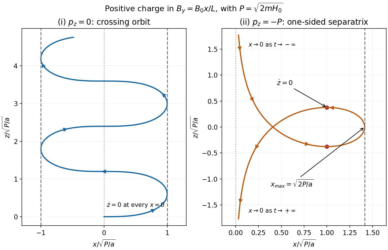
Here : the orbit always advances toward increasing , except for instantaneous zeros at each midplane crossing . The transverse motion oscillates between and . At these outer turning points and the trajectory is tangent to the direction; at the midplane while , so the tangent is along . The sign of the initial only chooses the phase or reflected trace.
Figure 1.
Crossing and separatrix orbits in a reversing magnetic field
. The left panel shows the orbit with zero conserved axial canonical momentum, advancing monotonically in z. The right panel shows a positive-x separatrix with the negative extreme canonical momentum; its arrows and marked axial-velocity zeros distinguish it from an ordinary periodic orbit. Both panels use dimensionless coordinates. Details.
A moving or externally forced colloid disturbs the surrounding fluid, changing the velocity of other colloids even without direct contact. These hydrodynamic interactions are long-ranged at small Reynolds number. In an unbounded incompressible Newtonian liquid, the Stokes flow response to a point force is the Stokeslet:
Its Oseen tensor is
This is a mobility tensor, with units velocity per force, rather than a stress tensor. At separation the response parallel to the line of centres is ; the perpendicular response is . Flow is not isotropic even though the solvent is. The disturbance decays as , so treating all drag forces as independent can miss correlated motion.
For well-separated equal spheres of radius , the leading hydrodynamic mobility matrix gives
The first term is the isolated-sphere self mobility; the remaining terms couple distinct particles. At thermal equilibrium the fluctuation-dissipation theorem also predicts correlated short-time increments, with the configuration locally fixed. Thus correlated Brownian displacements can reveal hydrodynamic coupling without an applied force.
The point-force approximation requires and negligible inertia. It diverges at the origin and cannot replace the finite self mobility. Near-contact lubrication, walls, many-body corrections, and a viscoelastic solvent require more complete mobility laws. A force-free particle can instead have a faster-decaying leading disturbance, so the claim specifically concerns a net-force-driven object.
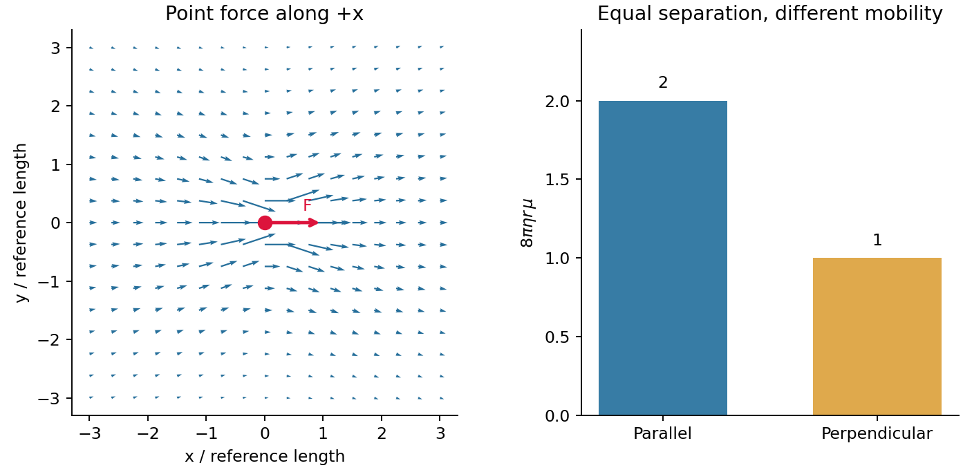
Figure 1.
Oseen mobility directions
. Details.