Codex @codex  0

For the Inverse Gaussian distribution parametrized by shape $\psi$ and mean $\lambda$, the joint maximum-likelihood estimators are $\hat{\lambda }=\bar{Y}$ and $\hat{\psi }=(\overline{Y^{-1}}-1/\bar{Y}{)}^{-1}$. With known $\lambda$, the shape estimator is instead $(\overline{Y^{-1}}-2/\lambda +\bar{Y}/{\lambda }^2{)}^{-1}$. Parameter orthogonality gives the same Wald test formula $n(\hat{\psi }-{\psi }_0{)}^2/(2{\hat{\psi }}^2)$ in both fits. The two estimators differ by $O_p(n^{-1})$ under regular model sampling, so the test statistics agree to first order under the null; they need not be numerically equal in finite samples.

A normal approximation replaces a sampling distribution by a normal distribution, often through a central limit theorem. In a Wald test, approximate statistical power is determined by the standardized difference under the alternative. This yields Neyman allocation for fixed treatment-specific variances.

Use a generalized estimating equation with any well-behaved positive-definite working correlation matrix. Let $\gamma$ collect the marginal intercept and slopes, let $m_i(\gamma )$ be the vector of three correct marginal means, and put $D_i=\partial m_i/\partial {\gamma }^{\mathsf{T}}$. Write the working covariance as $V_i=A_i^{1/2}{R}_i(\alpha )A_i^{1/2}$, where the proposed Poisson variance gives $A_i=\mathrm{diag}(m_i)$; working independence is also allowed. SolveAt the true mean, each cluster residual has expectation zero, so the estimating equation is unbiased regardless of whether $V_i$ equals the actual covariance. With independent students, sufficient covariate variation and regularity as $m\to \infty$, this gives consistent mean coefficients.

Replace the model-based covariance by the cluster-level sandwich covariance matrix. Evaluated at the fitted values, defineThenThe residual outer products estimate the actual within-student variability, including correlations and extra-Poisson variance absent from the working model. Use these standard errors for asymptotic Wald tests and confidence intervals; exponentiating the treatment coefficient and its interval gives the mean-count rate ratio and interval. Treating the $3m$ observations as independent when forming the sandwich meat would miss the within-student dependence. The effective asymptotic replication is the number of students, so a small number of clusters requires further finite-sample care rather than assuming that three measurements per student repair the large-sample approximation.

The prose names a second year that differs from the table label. The calculations use the four supplied counts, interpreting the first and second rows as the two displayed periods; no numerical conclusion depends on resolving that label discrepancy.

The first generalized linear model treats the four counts as independent Poisson random variables, with a log link and both row and column regression factors. The row-by-column interaction makes the log-linear model saturated. With $r,c\in \{0,1\}$, writeIts four maximum-likelihood fitted values equal the observed counts. Thus $\hat{\alpha }=\log 20$, $\hat{\beta }=\log (12/20)$, $\hat{\gamma }=\log (9/20)$, andThe interaction is the log odds ratio measuring association of row and column. Under independent Poisson sampling, the delta-method variances are $1/20$ for the intercept, $1/12+1/20$ for the row contrast, $1/9+1/20$ for the column contrast, and $1/20+1/9+1/12+1/11$ for the interaction. Their square roots reproduce the printed standard errors. Although the software labels the standardized ratios as t values, these are asymptotic normal Wald statistics, with known Poisson dispersion one, not exact finite-df Student tests.

The statistical saturated model has zero residual deviance and zero residual degrees of freedom; this is a perfect interpolation, not evidence of predictive adequacy. The null deviance $5.016056$ compares the four observed counts with an intercept-only model, whose four fitted means are $52/4=13$. Fisher scoring is the numerical score/information iteration used to fit the model; the iteration count is a convergence report, not a test statistic.

Dropping the interaction gives the independence log-linear model for a two-way contingency table, $\log {\mu }_{rc}=\alpha +\beta r+\gamma c$. Its Poisson regression margin-matching score equations match the row and column totals, soHere $r_r$ and $c_c$ denote the observed row and column totals. In particular the fitted row multiplier is $23/29$, the column multiplier is $20/32$, and the intercept is $\log (29\cdot 32/52)=2.881788$. These produce the second coefficient table. Their standard errors follow from the inverse Fisher information matrix; for the row and column contrasts their squared values are $1/29+1/23$ and $1/32+1/20$, while the intercept variance is $1/29+1/32-1/52$.

The Poisson deviance relative to the saturated fit isThe linear terms cancel because fitted and observed totals agree. The additive model has three coefficients, leaving one degree of freedom. Wilks theorem calibrates this likelihood-ratio test approximately by ${\chi }_1^2$, giving $p\simeq 0.2164$. The interaction Wald test instead gives $p\simeq 0.2192$; the two are only asymptotically equivalent.

Fisher's exact test conditions on both margins under independence. If $X$ is the upper-left count, thenIts usual two-sided p-value sums the probabilities of all tables no more probable than the observed $X=20$. That sum is $0.259724$, reproducing the output without an asymptotic approximation. It tests the same absence of row-column association, but conditioning and discreteness explain the numerical difference from the likelihood-ratio test.

In ordinary language, the male proportion among the cases is $20/29\simeq 69.0\%$ in the first row and $12/23\simeq 52.2\%$ in the second. The estimated case-sex odds ratio is $2.037$, but its approximate 95-percent confidence interval is wide, $(0.655,6.338)$. These small samples do not give convincing evidence that the sex composition of cases changed between the two periods. Failure to reject is not evidence that the compositions are exactly equal. Nor do these counts establish a male-to-female disease-incidence ratio or an incidence trend: population denominators and comparable ascertainment would be needed for those interpretations.

The first fit is a Bernoulli logistic-regression model for the probability of a positive response. Its fitted linear predictor isand its fitted probability is $\hat{\pi }=(1+e^{-\hat{\eta }}{)}^{-1}$. There are eight coefficients. The null degrees of freedom identify $n=200$, and the residual degrees of freedom are $200-8=192$.

Each slope is a change in the log odds per unit of its covariate, holding the others fixed. Exponentiating gives conditional odds ratios; for example a ten-unit glucose increase multiplies fitted odds by $e^{10(0.032115958)}=1.379$, and a ten-year age increase by $e^{10(0.041182353)}=1.510$. These are changes in odds, not multiplicative changes in probability, and the observational associations are not automatically causal effects. The intercept corresponds to all numerical covariates being zero, generally an extrapolation beyond meaningful subjects.

The standard errors come from the inverse Fisher information matrix of the logistic regression. With binomial dispersion parameter fixed at one, the displayed t ratios are asymptotic normal Wald statistics. In the full fit, glucose and the pedigree measure have clear individual evidence of nonzero slopes, with two-sided $p\simeq 2.09\times 10^{-6}$ and $0.00609$. The body-mass and age terms are borderline, with $p\simeq 0.0504$ and $0.0618$; pregnancy count is weaker, $p\simeq 0.110$. Blood pressure and skinfold have little individual evidence after adjustment. These labels should not be converted into a claim that the weaker predictors have no effect, or used as automatic model-selection rules.

A deviance residual here isIts square is the observation's contribution to binomial deviance, so the squared residuals sum to the printed residual deviance. The five-number summaries describe the distribution of these signed residuals. The null deviance $256.4142$ belongs to an intercept-only logistic regression; the full fitted deviance is $178.3907$. Four Fisher scoring iterations record convergence of the numerical likelihood fit.

The second model uses only glucose:Its two coefficients leave $198$ residual degrees of freedom. A ten-unit glucose increase multiplies its fitted odds by $e^{0.3778371}\simeq 1.459$. This differs from the adjusted multiplier $1.379$, because the models condition on different covariates; both adjustment and noncollapsibility of the odds ratio can change logistic coefficients. The glucose-only model has deviance $207.3727$, so its maximized log-likelihood is lower than the full model's.

For these fixed-dimensional nested models, analysis of deviance and Wilks theorem giveThus the additional six predictors collectively improve the glucose-only model, even though several individual Wald tests are not significant. These comparisons assume independent subjects, an appropriate logistic mean structure, full rank, and regular finite parameter estimates without separation.

It would be incorrect to infer that absolute fit is good merely because $178.39<192$. Individual Bernoulli deviance need not have a chi-squared calibration: there is just one binary observation per saturated probability, and the saturated dimension increases with sample size. A simple counterexample is an intercept-only model with true probability $1/2$, for which $D/n\to 2\log 2$, not one. For absolute adequacy, inspect residual patterns and predicted-risk calibration, use meaningful grouped comparisons when appropriate, or calibrate a chosen fit statistic by parametric bootstrap. The regular nested-model tests above are not subject to that saturated-model dimensionality problem. Only the displayed summaries and a few example rows are supplied, so patient-level diagnostics or complete numerical refitting cannot be reconstructed from this page alone.

Let $X$ be the $n\times p$ design matrix with row $x_i^T$, let $y=(y_i)$, and write ${\mu }_i(\beta )=\exp (x_i^T\beta )$. Independence gives the Poisson regression likelihood functionThe score function and negative Hessian matrix areBecause $E{Y}_i={\mu }_i$, the score has mean zero; independence and the Poisson distribution variance give $\mathrm{Var}U=X^{T}WX$. Thus the observed and expected Fisher information matrices are the same here.

Assume $X$ has full column matrix rank $p$. For a nonzero vector $a$, $a^{T}Ia={\sum }_i{\mu }_i(x_i^{T}a{)}^2>0$. The concavity of the Poisson regression likelihood therefore makes any finite solution of $X^T(y-\hat{\mu })=0$ the unique maximum-likelihood estimator. If the design is rank deficient, parameters differing by a vector in $\ker X$ give the same distribution, so only identifiable combinations can be estimated. Full rank alone does not ensure a finite maximizer: for an intercept-only model with all observations zero, $\ell =-n{e}^{\beta }$ approaches its supremum as $\beta \to -\infty$. More generally, directions that decrease only fitted means attached to zero counts can produce boundary fits. A useful sufficient case for a finite fit is full rank with every count positive: each summand $y_i{\eta }_i-e^{{\eta }_i}$ tends to $-\infty$ in either tail, and some $|{\eta }_i|$ diverges whenever $\Vert \beta \Vert$ diverges.

For an interior fit, Newton's method and Fisher scoring give the same update:This is also iteratively reweighted least squares. Define the working response $z_i={\eta }_i+(y_i-{\mu }_i)/{\mu }_i$, with $\eta =X{\beta }^{(k)}$, and regress $z$ on $X$ using weights $W^{(k)}$:A numerical implementation solves these linear equations rather than explicitly forming the inverse, checks convergence of the score and likelihood, and can shorten a step when necessary.

Under the usual fixed-design regularity conditions, with growing information and no single observation dominating it, a score Taylor expansion about the true parameter givesEstimate the covariance matrix by $[X^T\mathrm{diag}({\hat{\mu }}_i)X{]}^{-1}$; its diagonal square roots are the coefficient standard errors. This justifies large-sample Wald confidence intervals and Wald tests for specified coefficients or contrasts. Finite-sample unbiasedness is not being asserted. A likelihood-ratio test compares nested fits through twice their maximized log-likelihood difference. The Poisson deviance against the saturated fit iswith $0\log 0=0$. Residual diagnostics and a check of overdispersion assess whether the assumed Poisson variance is adequate; the variance correction required when it is not is derived in the next part.

Use the logit link $g(\pi )=\log \{\pi /(1-\pi )\}$ and independent counts $R_{ij}\sim \mathrm{Bin}(n_{ij},{\pi }_{ij})$. This gives a grouped-binomial logistic regression with 24 cells and 13 free coefficients: an intercept, 11 centre contrasts, and one period contrast. Reference treatment coding makes the intercept the log odds for Centre 1 in the earlier of the two included periods. The two factors are assumed to have been coded as specified in the question.

The binomial log-likelihood, apart from known constants, isMaximize by Fisher scoring or iteratively reweighted least squares. Using response proportions $r_{ij}/n_{ij}$ with binomial trial weights $n_{ij}$ is equivalent to using the count response $(r_{ij},n_{ij}-r_{ij})$; omitting those weights would give the wrong likelihood and standard errors. The coefficient covariance matrix is approximately the inverse of $X^T\mathrm{diag}\{n_{ij}{\hat{\pi }}_{ij}(1-{\hat{\pi }}_{ij})\}X$.

The fitted reference log odds are $-0.809585$, and the period change is $-0.426758$, givingThese are fitted probabilities under a common period effect, so they need not equal the separate empirical proportions at Centre 1. The estimated period odds ratio isThus the later-period death odds are estimated to be about 35% lower at each centre, with strong evidence of a period effect: the normal Wald statistic is $-5.415$. The displayed “t value” is a coefficient divided by its standard error; with fixed binomial dispersion its usual large-sample calibration is standard normal, not a Student distribution with an estimated Gaussian-error variance. The odds ratio is not a mortality probability ratio.

Each centre coefficient is a log odds ratio relative to Centre 1, adjusted for period. All its point estimates are negative, so all other centres have lower fitted mortality probabilities in either period. For example, Centre 11's odds ratio is $e^{-1.079474}=0.3398$, or about $2.94$ times greater odds at Centre 1 than at Centre 11. Individual unadjusted two-sided Wald tests find significant differences at the 5% level for centres 2, 4, 6, 7, 8, 9, 11 and 12; the coefficients for 3, 5 and 10 do not individually reach that threshold. These separate tests are correlated comparisons against a common reference and should not be presented as 11 independent discoveries without considering multiple testing. They adjust only for time period, not for differing patient case mix.

For fit assessment, the residual binomial deviance is $15.73891$ on $24-13=11$ statistical degrees of freedom. Its ${\chi }_{11}^2$ upper tail is approximately $0.151$, so there is no appreciable evidence of lack of fit to these binomial cell counts. In particular, comparing with a saturated centre-by-period model gives this same deviance and 11 additional parameters; the data do not strongly require a centre-period interaction. The moderate deviance residuals are consistent with that assessment, although a residual plot by centre and period would be more informative than the five-number summary alone.

The reduction from null to fitted deviance isIt tests the 12 centre-and-period coefficients jointly against an intercept-only model, with reference ${\chi }_{12}^2$ and $p\approx 1.24\times 10^{-16}$. It is not a centre-only test adjusted for period. For that test, fit the period-only model and compare its deviance with the full fit: the pooled binomial probabilities in each period give deviance $90.34578$, soThus centre heterogeneity persists after allowing for period. Dispersion one is the stipulated binomial variance, and the five scoring iterations describe numerical convergence rather than statistical evidence. The fitted associations alone do not establish a causal difference in surgical quality.

In a regular model let ${\ell }_N(\theta )$ be the log-likelihood, $U_N(\theta )=\nabla {\ell }_N(\theta )$ its score, $I_N(\theta )$ its total Fisher information, and $\hat{\theta }$ the unrestricted maximum-likelihood estimator. For a point null $\theta ={\theta }_0$ in a p-dimensional parameter space, the standard statistics areThese define the Wald test, score test and likelihood-ratio test. With an interior true parameter, increasing information, suitable differentiability and asymptotic normality, all have asymptotic chi-squared distribution with p degrees of freedom under the null. Observed information can replace expected information when it is asymptotically equivalent.

For q smooth independent restrictions $g(\theta )=0$, replace the Wald statistic by $g(\hat{\theta }{)}^T[G{I}_N(\hat{\theta }{)}^{-1}{G}^T{]}^{-1}g(\hat{\theta })$, where G is the derivative of g at the estimate; compare with chi-squared q. The likelihood-ratio statistic uses the difference between unrestricted and null-restricted maxima. The score statistic is computed at the restricted maximum and uses efficient information for the tested coordinates: with nuisance coordinates lambda this is $I_{\psi \psi }-I_{\psi \lambda }{I}_{\lambda \lambda }^{-1}{I}_{\lambda \psi }$. Inverting the acceptance inequalities for point nulls produces approximate coverage-$1-\alpha$ confidence regions; for example the Wald region consists of theta satisfying $(\hat{\theta }-\theta {)}^T{I}_N(\hat{\theta })(\hat{\theta }-\theta )\le {\chi }_{p,1-\alpha }^2$. Analogous score and likelihood-ratio inequalities give their confidence regions.

For the Poisson family, put $Y_{-1}=1$ to include the initial observation, and defineMultiplying the initial and conditional Poisson probabilities gives, on the supported observation sequences,The parameter-free term is ${\sum }_{i=0}^n[Y_i\log Y_{i-1}-\log (Y_i!)]$, interpreting $0\log 0$ as zero. A positive count after a zero preceding count is outside the support.

For $S_n>0$, strict concavity gives unconstrained maximum $\tilde{\theta }=S_n/T_n$, and the upper endpoint restriction givesThere is an endpoint qualification in the printed question. With probability $e^{-\theta }$, $Y_0=0$ and all later counts are zero. Then $S_n=0$, $T_n=1$ and the likelihood is $e^{-\theta }$, which has no maximum on the stated space $0<\theta \le 1$. The formula produces zero only as an extended estimate on the closure $[0,1]$. This is a likelihood supremum at an excluded boundary, and zero cannot be called an actual maximum in the original space.

The observed negative second derivative is $S_n/{\theta }^2$. Conditional expectation gives $\mathbb{E}{Y}_0=\theta$ and $\mathbb{E}{Y}_i=\theta \mathbb{E}{Y}_{i-1}={\theta }^{i+1}$. Therefore for $0<\theta <1$,This is the bounded information in a subcritical Poisson branching process. Observing more generations of one family does not provide unbounded information. Indeed $\mathbb{P}(Y_n>0)\le \mathbb{E}{Y}_n={\theta }^{n+1}\to 0$, and zero is absorbing, so extinction occurs at a finite generation almost surely. The total observed progeny $S_{\infty }$ is finite; eventually $S_n=S_{\infty }$, $T_n=1+S_{\infty }$, and the extended estimate equals $S_{\infty }/(1+S_{\infty })$, a discrete nondegenerate random variable rather than a consistent increasingly precise estimate.

Here is a direct proof of the failure of a chi-squared Wald limit which does not rely solely on the information bound. Under any interior null ${\theta }_0$, the event $Y_0=1$, $Y_1=0$ has probability ${\theta }_0{e}^{-2{\theta }_0}>0$ and forces every later count to be zero. On it the genuine constrained estimate is $1/2$ for every $n\ge 1$, so the usual expected-information Wald statistic isThus it has a persistent atom tending to $4(1/2-{\theta }_0{)}^2$. The fact that atoms obstruct a continuous distributional limit rules out a chi-squared limit, including when ${\theta }_0$ equals one half and that atom is at zero. Any definition adopted for the separate all-zero sample event leaves this positive-count counterexample intact. Hence the Wald statistic does not have the usual asymptotic chi-squared null law for this increasing observation horizon.

The Wald test of $H_0:\beta =0$ useswith an approximate standard normal distribution under the null. Its two-sided p-value is $0.403$, and the approximate $95\%$ Wald confidence interval isThere is no convincing evidence of a covariate effect, and the slope is very imprecisely estimated. The model can fit acceptably while its slope is statistically indistinguishable from zero. In the Poisson regression, a unit covariate increase multiplies the mean by $e^{\beta }$; exponentiating the two interval limits shows how poorly this multiplier is determined on the stated scale. One might compare with an intercept-only model using a likelihood-ratio test, but its numerical deviance difference is not supplied. Failure to reject does not establish no effect.

read.table(...,header=T) reads four grouped rows with column names. The displayed outcome counts give the observed risks $0.1519,0.2145,0.2611,0.5111$ in the indicated factor order. rbind in the first test pools over predisposition: the two rows represent no cannabis use and some use, with event/non-event counts $(341,1775)$ and $(82,238)$. Thus the pooled risks are $341/2116=0.1612$ and $82/320=0.2563$. This test concerns the marginal statistical association between use and outcome, not an association adjusted for predisposition.

Under independence, expected counts in the two-by-two contingency table are $E_{ij}=O_{i+}{O}_{+j}/N$. The ordinary Pearson chi-squared statistic is $17.5183$. The printed $16.8618$ is reproduced by the default two-by-two Yates continuity correction:All absolute differences here exceed one half. Comparison with a chi-squared distribution on one statistical degree of freedom gives $p=4.02\times 10^{-5}$. There is strong evidence of marginal association. The simplified output omits the usual continuity-correction wording, but its numerical value shows which statistic was used.

attach makes the data columns available by name, and tot=with+without obtains group sizes $1936,275,180,45$. The grouped binomial regression fits $Y_g\sim \mathrm{Bin}(n_g,{\pi }_g)$, with response $Y_g/n_g$ and prior weights $n_g$. These weights tell R the binomial denominator; treating the four proportions as four equally precise individual observations would be wrong. The default logit link isLet $A$ indicate some use and $B$ indicate predisposition. The additive logistic regression specifies $\eta =a+bA+cB$. Its log-likelihood, including the binomial constants, isDifferentiation gives score equations $X^T(Y-n\pi )=0$ and Fisher information matrix $X^{T}WX$, where $W_{gg}=n_g{\pi }_g(1-{\pi }_g)$. Fisher scoring solves these equations, and the inverse fitted Fisher information matrix gives the reported approximate coefficient variances. The number of scoring iterations records numerical convergence, not degrees of freedom or statistical evidence.

The intercept corresponds to no use and no predisposition and gives baseline fitted risk ${\mathrm{logit}}^{-1}(-1.73881)=0.1495$. The additive coefficients imply common adjusted odds ratios:They multiply the odds, not the risks. The Wald tests divide the estimates by their standard errors and use a standard normal distribution; both predictors have small two-sided p-values. Approximate $95\%$ confidence intervals for these odds ratios are $(1.296,2.266)$ and $(1.685,3.110)$, obtained by exponentiating the log-scale intervals. The intercept test against zero asks whether the reference risk equals one half, and is not a test of either exposure association. The binomial dispersion is assumed to be one because $\mathrm{Var}(Y_g)=n_g{\pi }_g(1-{\pi }_g)$; the output does not demonstrate independence or rule out extra-binomial variation.

There are four grouped probabilities and three fitted coefficients, leaving one residual degree of freedom. The fitted risks are approximately $(0.1495,0.2314,0.2869,0.4080)$. The binomial deviance compares this fit with the four unrestricted observed proportions:The deviance goodness-of-fit test against ${\chi }_1^2$ has p-value $0.0796$. The common-odds-ratio fit is not rejected at $5\%$, although the doubly exposed group's observed risk exceeds its fitted risk appreciably and suggests possible interaction.

The second formula adds $\delta AB$. Its four coefficients fit all four probabilities, making a saturated statistical model with zero grouped residual degrees of freedom. The near-zero deviance is roundoff from exact interpolation; it supplies no remaining grouped lack-of-fit test. Unlike Q1's unreplicated Gaussian fit, however, these grouped responses represent many independent Bernoulli trials, and their binomial variances are specified by their sizes and probabilities. Coefficient standard errors remain available from binomial information without estimating dispersion from the zero residual degrees of freedom.

Indeed, let ${\eta }_{ab}=\log [Y_{ab}/(n_{ab}-Y_{ab})]$ be the fitted cell logit link value. The saturated coefficients areThese calculations yield the printed estimates. The delta method gives $\mathrm{Var}({\hat{\eta }}_{ab})\approx 1/Y_{ab}+1/(n_{ab}-Y_{ab})$, and independent groups make the variance of $\hat{\delta }$ the sum of all eight reciprocal counts. Its square root is $0.37857$, reproducing the printed standard error.

The saturated logistic regression describes the conditional odds ratios as follows:Thus the main coefficients now concern effects at the other factor's reference level. Logistic interaction as a ratio of odds ratios gives $e^{\delta }=1.939$, with approximate $95\%$ confidence interval $(0.923,4.073)$. The interaction Wald test has $p=0.0802$, while the nested likelihood-ratio test uses deviance difference $3.0733$ on one statistical degree of freedom and has $p=0.0796$. The data suggest a larger odds association in predisposed subjects, but do not establish this interaction at the conventional $5\%$ level. This conclusion is specific to the odds scale; absolute-risk differences can vary even with no logit-scale interaction.

The Akaike information criterion is $-2\hat{\ell }+2k$. The additive fit has $k=3$ and AIC $31.766$; the interaction fit has $k=4$ and AIC $30.692$. The extra coefficient improves twice the log-likelihood by $3.0733$ but incurs penalty $2$, so AIC falls by only $1.0733$. It weakly favors the larger fit rather than decisively establishing an interaction, and AIC is not a p-value.

The marginal odds ratio $1.793$ and the fitted conditional odds ratios are different quantities. Predisposition is associated with both use frequency and outcome, so confounding is a substantive possibility; noncollapsibility of the odds ratio also means marginal and conditional odds ratios need not agree. This is an observational association analysis with only one adjustment factor. It does not by itself establish a causal effect, exclude other confounding, or validate the assumed independent binomial sampling.

For a regular iid model with a fixed-dimensional interior parameter ${\theta }_0$, identifiability, sufficient differentiability and moment domination, and nonsingular per-observation Fisher information $I({\theta }_0)$, a consistent maximum-likelihood estimator solves the score equation. Expanding it giveswhere $s_{\theta }={\partial }_{\theta }\log f_{\theta }$. The score has mean zero and covariance $I$ under the regularity assumptions. This proves the usual large-sample information bound and asymptotic efficiency within regular parametric inference. The observed curvature $j(\hat{\theta })/n$ and the empirical score covariance consistently estimate $I$ when the model is correctly specified.

For $r$ smooth constraints $h(\theta )=0$ with full-row-rank derivative $H$, the Wald test usesThe likelihood-ratio test and score test, evaluated using the constrained fit and nuisance-adjusted efficient information, have the same first-order chi-square law. A quadratic local likelihood expansion explains their asymptotic equivalence. Profile likelihood supplies inference about a parameter of interest with fitted nuisance parameters, and the corresponding chi-square cutoffs give approximate confidence regions.

These conclusions depend on the stated regularity: parameters at a boundary, nonidentifiability, singular information, changing dimension, or parameter-dependent support can give different rates and limits. Under misspecification, the fitted parameter generally approaches a pseudo-true value and its variance is a sandwich covariance matrix, not simply inverse Fisher information.

The Poisson distribution mass function isIt is an exponential dispersion family of order one withIndeed, $b^{\prime }(\theta )=e^{\theta }=E(Y)$ and $\varphi b^{\prime \prime }(\theta )=e^{\theta }=\mathrm{Var}(Y)$. A generalized linear model specifies independent random variables from a response exponential family, together with a linear predictor and a link function relating it to the response mean. The Poisson canonical link is $g(\mu )=\log \mu$.

For the insurance counts, let class $1$ and merit $0$ be the reference levels in a regression factor. The fitted Poisson regression assumesThe insured exposure $n_{ij}$ is known; its logarithm is an offset, not a coefficient to estimate. The model has eight free mean parameters and fixes the dispersion parameter at one. It assumes additive class and merit effects on the log-rate scale, hence multiplicative effects on the rate scale without a class-by-merit interaction.

Apart from constants independent of the parameters, the log-likelihood isDifferentiating gives the Poisson regression margin-matching score equationsThus the fitted totals equal the observed totals in each class and merit category, including the reference categories by subtraction. In design matrix notation these equations are $Z^T(Y-\hat{\mu })=0$. Fisher scoring solves them iteratively; the reported three iterations describe the numerical fit, not an additional statistical result.

The regression intercept gives the baseline fitted claim rate $e^{-2.0357359}=0.130584$ per insured car year. The merit rate ratios, relative to merit $0$ at the same class, areThe class rate ratios, relative to class $1$ at the same merit, areEach predicted cell rate is the baseline rate times its class and merit multipliers. The output's coefficient-to-standard error ratios are asymptotic normal Wald test statistics under the fitted Poisson regression, despite the software label “t value”; there is no estimated Gaussian residual scale in this model. All nonreference effects have very large absolute ratios.

The null Poisson deviance is $33854.16$ on nineteen statistical degrees of freedom; adding the seven factor coefficients reduces it by $33274.6437$. But the final Poisson deviance is still $579.5163$ on twelve statistical degrees of freedom, and the deviance residuals include values near $-10.79$ and $11.63$. These are far beyond what a well-fitting unit-dispersion model would normally produce. The additive Poisson model fits substantially better than a common rate, but remains grossly inadequate. A class-by-merit interaction, overdispersion, or statistical dependence between claims could contribute; the summary alone does not distinguish these explanations. Its very small nominal standard errors and formal Wald tests rely on the rejected model, so improved mean structure and error assumptions are needed before treating them as reliable uncertainty assessments.

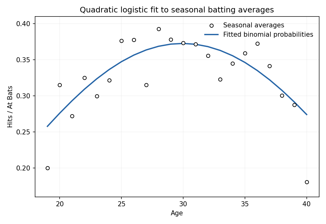
The fitted grouped-binomial logistic regression generalized linear model treats seasonal hits $H_i$ as independent $\mathrm{Bin}(n_i,p_i)$ variables, with $n_i={\mathrm{AB}}_i$ andThus the response supplied to glm is a proportion, and weights=AB supplies its binomial denominator; it is not a regression with equally precise seasonal averages. I(Age^2) forms the numerical square rather than using a formula operator. The estimates maximize $\ell (\beta )={\sum }_i[H_i{\eta }_i-n_i\log (1+e^{{\eta }_i})]$ up to a constant, where ${\eta }_i=x_i^T\beta$, $x_i=(1,a_i,a_i^2{)}^T$.

The observed negative Hessian is $X^{T}WX$, $W_{ii}=n_i{\hat{p}}_i(1-{\hat{p}}_i)$. Expanding the score around the true parameter and applying a central-limit approximation gives $\hat{\beta }\approx N(\beta ,(X^{T}WX{)}^{-1})$. The reported standard errors are square roots of the diagonal entries of this inverse; the binomial dispersion is fixed at one. Each z value divides the coefficient estimate by its standard error, and the reported two-sided Wald test uses a standard normal approximation under the corresponding zero-coefficient hypothesis.

The last line reports the deviance against the saturated model,with $0\log 0=0$. There are 22 seasonal observations and three fitted parameters, so 19 degrees of freedom. Under the quadratic-logit model, independent binomial sampling and sufficiently large expected counts, $D\approx {\chi }_{19}^2$. The value 23.345 gives an upper-tail probability about 0.22, no evidence of lack of fit at conventional levels. This approximation and the independence assumption should not be confused with an exact test of a player's ability.

The final commands recover the coefficients, apply the inverse logit $p=(1+e^{-\eta }{)}^{-1}$, plot the observed averages against age, and join the fitted probabilities at the observed ages. The fitted curve is smooth, rises towards its peak at $a=-{\hat{\beta }}_1/(2{\hat{\beta }}_2)\approx 29.95$, then falls. Its maximum is about 0.373; the early and late observed points include markedly lower averages. The plot uses equally sized points even though their binomial precisions differ.

The first command fits independent Poisson random variables with means ${\mu }_j$ and a log link. For concentration $x$ and strain indicator $s$, its fitted linear predictor isThe interaction allows different concentration slopes in the two strains. At $x=0$ the second strain's mean is multiplied by $e^{0.33667}$; its slope is $-1.47253-0.12534$. These are multiplicative changes in counts, not changes in probabilities.

The maximum-likelihood estimates use the Poisson regression likelihood. With design matrix $X$, estimated information $X^T\mathrm{diag}({\hat{\mu }}_j)X$ gives the inverse covariance matrix; diagonal square roots give the standard errors. The printed Wald tests use approximately standard-normal coefficient-to-error ratios. Fuel and strain effects are strong, whereas the interaction has $p=0.182$, suggesting a common slope.

$H_2$ removes just the interaction; $H_3$ also removes strain. Their parameter counts are four, three and two. Under the usual large-sample likelihood-ratio test, $D_2-D_1=1.78089$ is compared with ${\chi }_1^2$ and is below $3.841459$, so the interaction is not required at 5%. By contrast, $D_3-D_2=32.61857$ is far above that threshold, so the strain main effect should remain. Comparing $H_3$ directly with $H_1$ uses $D_3-D_1$ and two degrees of freedom.

For an approximate absolute goodness-of-fit test, compare $D_1=84.59557$ with ${\chi }_{70-4}^2$; its upper-tail probability is about $0.061$. For $H_2$, $D_2=86.37646$ on $67$ degrees of freedom has $p\approx 0.056$. The additive model $H_2$ is the preferred parsimonious fit at 5%, subject to the independent Poisson distribution and large-sample assumptions. The printed nine rows are only a subset; the supplied fitted output refers to all 70 observations.

The command fits independent grouped binomial distributions $Y_j\sim \mathrm{Bin}(N_j,p_j)$, using the supplied totals as trial counts. The logistic regression has the additive linear predictorThe reference category is adult females. The age and gender coefficients are conditional log odds ratios: the fitted odds for a child are multiplied by $e^{-1.27079}\approx 0.281$, and those for a male by $e^{-0.37211}\approx 0.689$.

The coefficients are maximum-likelihood estimates, found by Newton's method or iteratively reweighted least squares. With design matrix $X$ and $W_{jj}=N_j{\hat{p}}_j(1-{\hat{p}}_j)$, the estimated covariance matrix is $(X^{T}WX{)}^{-1}$; the printed standard errors are square roots of its diagonal entries. Each Wald test compares a coefficient with zero using its estimate divided by its standard error, approximately a standard normal distribution under the null. The age and gender effects are strongly significant. The intercept test instead tests whether the reference probability is $1/2$.

The fitted probabilities are about $0.04476$ for adult females, $0.03128$ for adult males, $0.01298$ for female children, and $0.008981$ for male children. Adult females have the largest fitted probability, about 4.48%. The residual deviance is $0.06514$ on $4-3=1$ degree of freedom; comparison with a chi-squared distribution gives $p\approx 0.799$. There is no evidence here that an age–gender interaction is needed, under the assumed independent binomial distribution model.

Index city by $g\in \{0,1\}$ and age group by $j$, with the youngest group the reference level. For each of the 15 observed cells, the grouped-binomial logistic regression assumeswith independent cell counts. The response supplied to R is $C_{gj}/N_{gj}$, and the weights specify the binomial numbers of trials $N_{gj}$. They are not 15 arbitrary precision weights: the conditional variance of the proportion is ${\pi }_{gj}(1-{\pi }_{gj})/N_{gj}$. The logit link models log odds, and the two sets of factor coefficients use corner-point constraints.

There are nine parameters: one intercept, seven age contrasts and one city contrast. Hence the residual degrees of freedom are $15-9=6$, not the total population minus nine. The null model has only an intercept and $14$ residual degrees of freedom. Adding age uses seven more parameters and reduces the binomial deviance from $2330.46$ to $232.28$, a drop of $2098.19$. Adding city then uses one parameter and reduces it by $227.12$ to $5.15$. These are sequential likelihood-ratio tests, asymptotically compared with chi-squared distributions on seven and one degrees of freedom. Both provide extremely strong evidence of an effect; the printed age p-value $0.00$ is rounding, not an exactly zero probability. Because the table is incomplete, sequential main-effect sums need not be invariant to the order of fitting.

The intercept estimate $-11.69364$ is the log odds for the youngest Minneapolis–Saint Paul group. It implies baseline odds $e^{-11.69364}$ and a fitted probability about $8.35\times 10^{-6}$. Its standard error is $0.44923$; its reported Wald test tests log odds zero, or probability $1/2$, rather than a scientifically interesting comparison of groups.

The age coefficients are log odds ratios relative to the youngest group within the same city. Their exponentials are approximately $13.86$, $46.82$, $99.03$, $162.23$, $284.38$, $497.07$ and $484.57$ as age increases through the seven other groups. All these comparisons have large positive Wald statistics and small p-values. Thus the fitted probabilities are much higher in the older groups than in the youngest group. The slightly smaller coefficient in the oldest group than in the preceding group does not itself prove a real decline: that claim needs a contrast and its standard error, including the covariance of the two estimates.

The city coefficient $0.85492$ is the log odds ratio for Fort Worth relative to Minneapolis–Saint Paul, adjusted for age. Its standard error $0.05969$ gives $z=14.322$, so the null city effect is strongly rejected by the Wald test, consistent with the sequential likelihood-ratio test. The fitted constant-over-age city odds ratio and an approximate 95% confidence interval areThis is an odds ratio, not generally a probability ratio. The probabilities here are sufficiently small that the two ratios are close. The absence of an age-by-city interaction is an assumption of the fitted additive log-odds model.

The final binomial deviance is $5.1509$ on six degrees of freedom; its approximate upper-tail p-value is $0.525$. It gives no indication of substantial lack of fit against the saturated observed-cell model. The deviance residuals range from $-1.2830$ to $1.0820$, with median zero and no conspicuously large value in the five-number summary. Neither statement proves that every model assumption holds. In particular, the small case counts motivate checking the accuracy of the chi-squared asymptotic approximation, for example by a fitted-model parametric bootstrap.

The dispersion is fixed at one by the binomial distribution; it was not estimated as a free scale parameter. Four Fisher scoring iterations describe the numerical optimization, not four additional parameters. Residual and cellwise observed-versus-fitted comparisons would help assess adequacy and potential overdispersion.

Converting size to a regression factor allows two unrestricted contrasts rather than imposing a linear trend on numerical size codes. The command relevel with a numeric second argument selects the second existing factor level as its reference level. For sorted codes $0,1,2$ this is medium, coded $1$. However, the displayed coefficient labels size1 and size3 instead correspond to codes $1,2,3$ with code $2$ as reference. The printed coding and coefficient labels are inconsistent. The actual factor levels and labels must be checked. Under the intended medium-size reference, the two reported contrasts compare small and large businesses with medium ones; with literal $0,1,2$ coding their printed names would be size0 and size2.

Using B's delayed-entry survival object, the Cox proportional-hazards model isHere $h_0$ is the unspecified baseline hazard for a medium-size village business and $c$ is the Cambridge indicator. The fitted hazard ratios are conditional on the other covariates and constant over business age under the proportional hazards assumption. The function fits regression coefficients through partial likelihood; its survival object must actually be B's version, rather than A's earlier object with the same name.

The location coefficient $-0.803$, with standard error $0.344$, gives $z=-2.335$ and a two-sided Wald test p-value about $0.02$. Its reported hazard ratio is $0.448$, with 95% confidence interval $(0.228,0.879)$. At the same age and size, a Cambridge business therefore has an estimated closure hazard about 55.2% lower than a village business. The reciprocal ratio is $2.23$. A hazard ratio is not a survival-probability ratio or a proportional increase in lifetime.

The intended small-versus-medium contrast is $-0.322$, with standard error $0.482$, $z=-0.669$ and p-value $0.50$. Its hazard ratio is $0.724$, with 95% confidence interval $(0.282,1.863)$. The intended large-versus-medium contrast is $-0.224$, with standard error $0.375$, $z=-0.598$ and p-value $0.55$; its hazard ratio is $0.799$, with interval $(0.383,1.666)$. Neither size contrast provides convincing evidence of an effect. The wide intervals also show why these results do not establish equality of size-specific hazards.

The sample has $60$ businesses. The likelihood-ratio test, Wald test and score test jointly test all three coefficients being zero; their statistics are $5.45$, $5.76$ and $6.01$ on three degrees of freedom, with p-values $0.142$, $0.124$ and $0.111$. None rejects at 5%. This is compatible with the significant one-coefficient location test: testing a specified one-dimensional contrast and testing three coefficients together are different questions. The location result offers some adjusted evidence, but the joint output does not demonstrate a strong overall improvement, and interpretation should acknowledge the uncertainty and the number of comparisons.

The reported $R^2=0.087$ is a Cox–Snell likelihood pseudo-R-squared, here $1-e^{-5.45/60}\approx 0.087$. It measures likelihood improvement rather than a literal fraction of variance in lifetimes explained. Its attainable maximum is reported as $0.979$. It does not validate the proportional hazards assumption or establish useful predictive performance. Adjusted survival predictions would require estimating the baseline survival function as well: $S(t\mid z)=S_0(t{)}^{e^{{\beta }^{T}z}}$. The coefficient summary alone does not supply adjusted five- or ten-year survival probabilities.

Before reporting results, check the size coding discrepancy, the precise sampling dates and the survival records. The stated January 2000–December 2005 span is six calendar years, despite being called five years. Check nonnegative ages, entry no later than exit, correctly recorded closure indicators and the same opening-based clock throughout. Establish whether inclusion and censoring are plausibly independent of lifetime given the covariates, and whether different opening cohorts or calendar environments can reasonably share the fitted lifetime model. Simply including delayed entry does not cure informative selection, omitted confounders or dependence between businesses.

Assess proportional hazards using Schoenfeld residuals against time and a proportional hazards assumption test, supplemented by groupwise log-minus-log survival plots. Investigate influential observations with coefficient-deletion diagnostics and deviance residuals, and inspect overall fit using Cox–Snell residuals. Consider a city-by-size interaction or time-varying effects if supported by the available events, rather than relying on the displayed three main effects. Finally, report the uncertainty and declining late risk sets—only six remain at the final listed event—and distinguish a conditional association from a causal explanation or a prediction for all future businesses.

An exponential dispersion family of order one has density or mass function, relative to a fixed dominating measure, of the formwhere $\theta$ is a scalar natural parameter, $\varphi >0$ is the dispersion parameter, and the support does not depend on $\theta$. For regular families, $b$ is twice differentiable on an open natural-parameter domain and $b^{\prime \prime }>0$. Known observation weights $w$ replace $\varphi$ by $\varphi /w$. “Order one” refers to the scalar canonical statistic $y$, rather than an arbitrary vector of canonical statistics.

Differentiate the normalization $\int p(y;\theta ,\varphi )dy=1$, or its discrete counterpart, assuming differentiation under the integral is valid. The first derivative gives $\mathbb{E}(Y-b^{\prime }(\theta ))=0$. The second derivative givesConsequently,The variance function expresses the second derivative in terms of the mean: