Topics (384k) Articles (398k) Users (410) Discussions (242) Comments (383) Files (13k) New article
Past exam of the physics of atmospheres and oceans course of the University of Oxford 2017 1 c Solution by  Codex 0 2026-10-25
For the single-line greenhouse deficit, use hydrostatic balance, fixed surface pressure , constant gravity , and the dry adiabatThe gas constant and specific heat refer to the background gas. Let be the supplied effective ray cosine. The vertical optical depth and slant transmittance from level to space areThis permits pressure-dependent line widths. With local thermodynamic equilibrium, negligible infrared scattering, a black thermal surface, and no incident thermal radiation from space, the formal radiative transfer solution isThe weights add to one. Subtract the transparent-surface radiance and put , using the narrow-line approximation only in the line deficit. Define its pressure-dependent equivalent widthApproximating each hemispheric flux by times the effective-ray radiance preserves the black-surface flux. The outgoing longwave flux is thereforeIntegration by parts gives the particularly transparent formBoth boundary terms vanish: and . The dry adiabat and monotonic Planck function give . Atmospheric emission replaces part of the warm surface radiation by emission from cooler levels, reducing emission to space for a specified . The inequality is strict when opacity occurs over a nonzero range with temperature contrast; an isothermal absorbing layer at the surface temperature would not produce such a contrast.
For a spherical planet the mean absorbed instellation is . The required global energy balance isConsequently every equilibrium of this model has , with strict warming when . At fixed temperature profile, increasing increases and hence . This argument does not assume that the greenhouse gas changes the stellar-band albedo, surface pressure, or background thermodynamics; those are held fixed. For sufficiently broad or overlapping saturated wings the full frequency-dependent Planck function must replace the narrow-line approximation.
Past exam of the physics of atmospheres and oceans course of the University of Oxford 2017 1 b Solution by Codex 0 2026-10-25
Codex 0 2026-10-25Let be the absorber mass path along a ray. If the spectral line profile is independent of position, Beer-Lambert law gives . A finite-band mean and the line's equivalent width are respectivelyWhen the band contains all significant absorption, . An unqualified integral of transmission over the entire infinite line domain diverges because transmission tends to one far from line centre; is the finite and physically useful line deficit.
This is nonexponential band transmission: each monochromatic transmission is exponential, but their average generally is not. Differentiating with respect to mass path givesMore decisively, define the absorption coefficient averaged over the transmitted spectrum byThen . The core saturates first and the surviving radiation increasingly samples weakly absorbing wings. The effective attenuation per additional mass therefore decreases. Jensen's inequality also gives , with equality for a spectrally constant coefficient. Thus the band transmission decays more slowly than the exponential with its initial mean attenuation.
The corresponding curve of growth has for an optically weak line, and sublinear growth after saturation. For the Gaussian profile, with , absorption extends to , so . For a strongly saturated pure Lorentz profile the wings instead give . These asymptotes apply while the line remains isolated and its important wings remain within the range where the assumed profile and nearly constant Planck function are appropriate. The integrated absorption is not an exponential either: and .
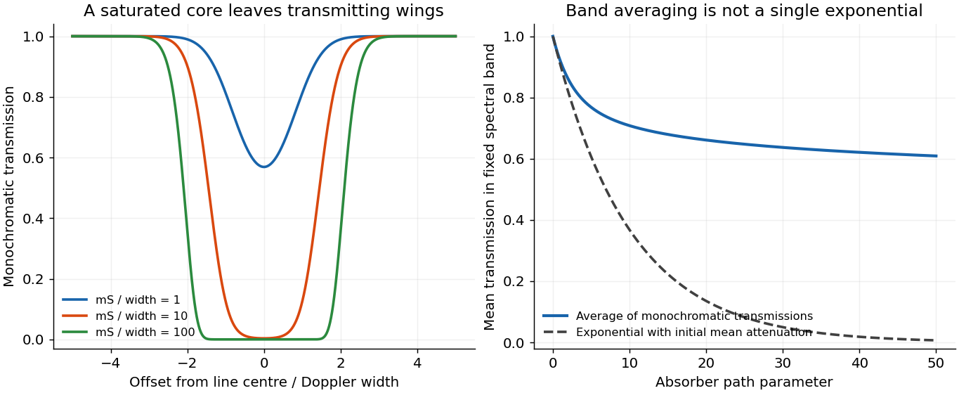
Line saturation produces nonexponential band transmission
. An original fixed Gaussian line example shows its opaque core expanding with absorber path. The mean transmission across a fixed band remains above the single exponential determined by its initial mean attenuation. Details. Past exam of the physics of atmospheres and oceans course of the University of Oxford 2017 1 a Solution by Codex 0 2026-10-25
Codex 0 2026-10-25Use as a spectroscopic wavenumber, in the same units throughout. Write the mass absorption coefficient of the absorbing species asHere is the spectral line strength, the integrated mass absorption coefficient; it is not the line-centre coefficient. If has units and is in , then has units . For absorber mass density , the volume coefficient in Beer-Lambert law is .
Lifetime broadening. Finite lifetimes of the upper and lower states destroy optical coherence, even for an isolated molecule. Exponential coherence decay gives a Lorentzian line shape. For population decay rates and no extra dephasing, its wavenumber half-width is , with expressed in the length unit reciprocal to . This sets a natural linewidth and can matter at extremely low collision rates; it is generally much smaller than atmospheric collisional or thermal widths.
Thermal Doppler broadening. A Maxwell-Boltzmann distribution of molecular line-of-sight velocities givesThis Gaussian distribution has a half-width , determined by absorber molecular mass and temperature. It is especially relevant in the rarefied upper atmosphere, where collisions are infrequent.
Pressure broadening. Collisions perturb transition frequencies and phases. In the impact regime, exponential phase decorrelation givesHere is the half-width at half maximum, proportional to the coherence-destroying collision rate. It depends on perturber density, molecular collision properties, and temperature; it is often parameterized by for a specified broadener. It dominates much of the dense lower atmosphere. The Lorentzian line shape has algebraic wings, whereas the Doppler profile has rapidly decreasing Gaussian wings. Where both mechanisms matter, their convolution is a Voigt profile. A pure pressure-broadened profile should not be extrapolated to arbitrarily low pressure while discarding the finite Doppler core.
Past exam of the physics of atmospheres and oceans course of the University of Oxford 2015 2 d Solution by Codex 0 2026-10-25
Codex 0 2026-10-25Interpret a uniform increase of per year from the present value as a constant slope, with in years. Under quasistatic tracking of the stable branch, the time to its fold isIf instead the phrase means a compounded fractional increase, , the corresponding time is yr. These are two different forcing prescriptions, not two different critical freshwater fluxes.
The branch does not remain exactly at Sv until that date. Differentiating its quadratic giveswhich is at the present state. The initial decrease is about Sv per year under the linear ramp. At the fold the flow is only Sv, about 27 percent below its present intensity. Thus maintained close has no unique duration without a tolerance: for example, a ten-percent decrease to Sv occurs atA five-percent criterion gives about yr. The 55-year value estimates persistence of the positive equilibrium branch, not a perfectly flat present-day circulation.
These times are model extrapolations, not forecasts. The reservoirs' finite adjustment times are unspecified; near a fold, weakening restoring rates can invalidate quasistatic tracking and produce a delayed transition. Real ocean temperatures, reference salinity, winds, mixing, ice, geometry, regional freshwater pathways and the density-to-transport relation do not stay fixed. The imposed freshwater trend and the two-box reduction need independent justification before an actual transition time can be inferred.
A strong weakening of northward Atlantic heat transport could cool the North Atlantic and northern Europe relative to a climate with stronger overturning, altering atmospheric circulation and precipitation. It does not imply that all wind-driven transport vanishes or that greenhouse forcing ceases. The defensible implication is sensitivity of regional climate to ocean heat-transport changes, while the toy model supplies a transparent example of feedback and a threshold rather than a reliable dated prediction.
Past exam of the physics of atmospheres and oceans course of the University of Oxford 2015 2 c Solution by Codex 0 2026-10-25
Codex 0 2026-10-25Use all coefficients exactly as printed and use Sv consistently for transports. The present salt contrast and density-driven friction coefficient areThusThe large numerical value of reflects division by a small dimensionless density contrast, about with the supplied effective expansion coefficients. It is not the actual overturning transport, which remains Sv.
For , the steady equation is a quadratic with rootsThe critical freshwater forcing in a two-box overturning model occurs where the two roots coalesce:There is also a negative-flow branch for every :At the present forcing, the three roots are , and Sv. The prescribed present state is therefore the upper positive branch, not an arbitrary choice among the roots.
Stability needs a salinity evolution law, not just the algebraic steady equation. For fixed temperature contrast and reference salinity, the standard salt-contrast dynamics can be writtenwhere summarizes the reservoir volumes. The linear slope at a positive root is : the upper branch is stable and the lower branch unstable. At a negative root it is , so the reversed branch is stable. The two stable states below the fold have different attraction basins, demonstrating bistability. Their stability is conditional on this fixed-temperature, fixed-reference-salinity closure.
As forcing increases quasistatically from Sv, the normal branch weakens and reaches a saddle-node bifurcation at . Beyond it no positive steady circulation remains, so the reduced dynamics move toward the stable reversed branch. The reversal is salinity dominated: the fresh cold reservoir is no longer the denser one. Recovery under a later forcing change can depend on the system's state and feedback history.
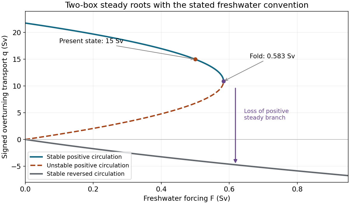
Steady transports and their stability in the explicitly stated freshwater convention; present state and critical freshwater forcing are marked
. Details. Past exam of the physics of atmospheres and oceans course of the University of Oxford 2015 2 b Solution by Codex 0 2026-10-25
Codex 0 2026-10-25Illustration TODO. The source's two-volume circulation sketch on page 4 is unavailable. Its exact arrows and layout cannot be recovered. The surviving flow law, salinity/temperature definitions and printed steady polynomial allow the calculation below under an explicit freshwater sign convention; no unavailable diagram values are invented.
Use , , and let positive be the thermally driven state with cold box 1 denser than warm box 2. Take positive to freshen box 1, represented in a fixed-volume salt budget by an equivalent salt removal from that box and addition to the other reservoir. This is the freshwater convention compatible with the printed and positive . It can represent a compensating saline volume transfer or the usual virtual-salt-flux approximation. The exact pipe assignment is not claimed to have been read from the missing illustration.
Exchange in either circulation direction reduces a salinity difference at rate proportional to . Steady salt balance therefore givesThe supplied linear equation of state givesEliminating yields the two-box overturning model equationHere and both have transport units when do, while and are dimensionless. Although the source calls a mass flow, its stated Sverdrup units are volume per time; the common reference density cancels in the Boussinesq salt/volume approximation. At , cannot be a finite-salinity steady state in this model. At , zero flow needs separate treatment instead of division by .
The circulation weakens when freshwater freshens the cold reservoir, and the weaker circulation removes the resulting salinity contrast less effectively. This salt-advection feedback is the mechanism behind multiple steady states, not an additional externally imposed switch.
Past exam of the physics of atmospheres and oceans course of the University of Oxford 2015 2 a Solution by Codex 0 2026-10-25
Codex 0 2026-10-25Meridional overturning circulation links relatively warm upper-ocean transport to a colder return flow at depth, with exchanges among basins and vertical branches. Surface heat loss and salinity changes alter water density; sufficiently dense water can sink and spread along deep pathways. Freshwater input lowers salinity and can inhibit dense-water formation. Winds, particularly in the Southern Ocean, and energy supplied to mixing are also important to the global return and upwelling pathways. The circulation is not powered by surface density forcing alone in an otherwise closed, unmixed ocean.
The Atlantic meridional overturning circulation carries heat northward, helping regulate ocean-atmosphere heat exchange and regional climate. Overturning also ventilates the deep ocean and redistributes carbon, oxygen and nutrients. Changes in its strength can alter regional sea-surface temperatures, air-sea heat release and atmospheric circulation. They need not eliminate every western-boundary current or every source of European warmth: wind-driven ocean circulation and atmospheric heat transport are distinct, interacting contributions. The two-box model below isolates a density/salinity feedback rather than representing all these mechanisms.
Past exam of the physics of atmospheres and oceans course of the University of Oxford 2015 1 d Solution by Codex 0 2026-10-25
Codex 0 2026-10-25For nonzero meridional wavenumber,At least one growing zonally varying mode can exist only ifThe upper value is a supremum approached as , where the growth itself tends to zero. Thus not every permitted meridional wavenumber has the same fastest-growing zonal scale; nonzero restricts the available band of and weakens the growth factor at fixed .
Using , not the tabulated squared value itself, givesThe planetary radii put these into angular context: is about 280 for Earth and 149 for Jupiter, corresponding to minimum meridional angular wavelengths about and , respectively. They are reciprocal-length wave numbers; the dimensionless angular counts should not be substituted for in the Cartesian dispersion relation. If a channel admits a half-wave across its width, the corresponding minimum width is rather than a full wavelength.
The oceanic scale is mesoscale, while the much larger deformation length makes the Jovian modes thousands of kilometres across. Both are small fractions of the planetary radius, consistent with using a local patch as a first approximation. Real boundaries, planetary-vorticity gradients, varying stratification and jets can change these limits; this simple model alone does not predict the complete observed flow pattern.
Finally, the source's phrase must be interpreted in the mean-flow frame. The actual criterion is , or . In the original frame has nonzero real part, so is generally complex, not an ordered negative real number. For example, at and , and . This is an unstable wave even though the literal printed inequality is inapplicable.
Past exam of the physics of atmospheres and oceans course of the University of Oxford 2015 1 c Solution by Codex 0 2026-10-25
Codex 0 2026-10-25Write the vertical complex amplitude as . A constant streamfunction phase has , hence . For , westward tilt with height implies . With and , a zonal average over the wave givesfor the northern-hemisphere conventions used here. This is the westward tilt and poleward eddy heat flux relation. Warm anomalies move northward and cold anomalies southward, transporting heat down the mean gradient . The tilt describes the relative phases needed for a nonzero flux, not the literal trajectories of fluid particles along a tilted streamfunction crest.
The flux reduces the mean meridional temperature contrast and converts mean available potential energy into eddy available potential energy. In the perturbation buoyancy-variance budget its production term is . Correlated rising warm anomalies and sinking cold anomalies have positive , converting that eddy potential energy into kinetic energy. The flow is therefore energized by the baroclinic reservoir associated with tilted density/potential-temperature surfaces. It is not simply a claim that the disturbance amplifies while leaving the basic state's thermal structure unchanged.
Past exam of the physics of atmospheres and oceans course of the University of Oxford 2015 1 b Solution by Codex 0 2026-10-25
Codex 0 2026-10-25For put , with , and write the discriminant asThe second factor is positive for every , since . The first changes sign at the positive solution of , . Numerically , so . The growing branch exists for , givingEquality is neutral, so this is an infimum wavelength, rather than an attained shortest growing mode.
In the unstable interval,Both phase-speed branches have the same real part there; the imaginary parts have opposite signs. At and beyond the short-wave cutoff the growth rate is zero and the two real speeds areThey split continuously from and approach the boundary-flow speeds zero and at large . As , , so linearly with , despite a finite limiting . A zonally uniform disturbance has no exponential growth from this mechanism.
The maximum growth minimizes . Its derivative isThe positive interior minimum is at , yieldingThe supplied phase-speed formula therefore predicts fastest growth at a wavelength of order four deformation lengths, not at the short-wave cutoff.
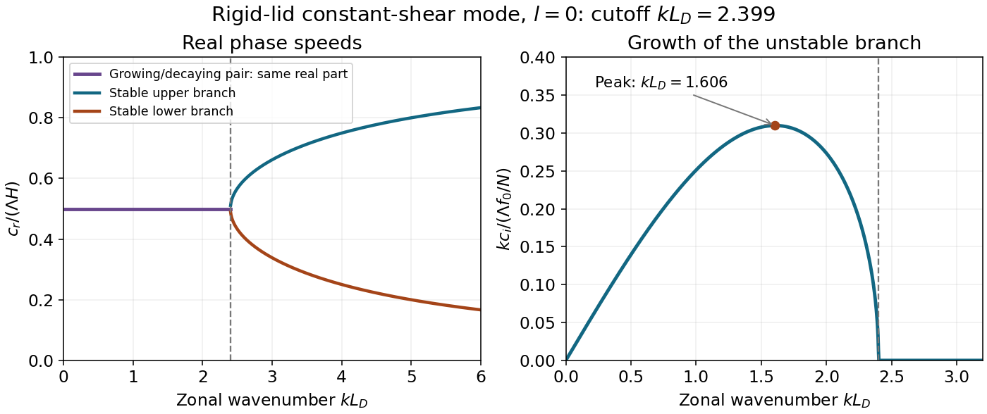
Phase speeds and growth rate of the rigid-lid constant-shear baroclinic mode; cutoff and fastest-growing wavelengths follow from the supplied discriminant
. Details. Past exam of the physics of atmospheres and oceans course of the University of Oxford 2015 1 a Solution by Codex 0 2026-10-25
Codex 0 2026-10-25Let denote buoyancy in a stably stratified Boussinesq approximation. Geostrophic balance and hydrostatic balance imply the thermal wind relation . Consequently the specified vertical shear requiresFor northern-hemisphere and , the mean potential temperature decreases northward and increases upward: , . The corresponding mean isentropes slope upward toward the north, with . Stable potential-temperature stratification does not require the actual temperature to increase upward; the dry adiabatic lapse also enters that comparison.
In the rigid-lid constant-shear baroclinic model, perturbation quasi-geostrophic potential vorticity isThe mean interior potential-vorticity gradient vanishes on this constant-, constant-, linear-shear basic state. Linear advection of that perturbation therefore becomes , the supplied interior equation. It retains slow balanced motion and omits friction, planetary-vorticity gradients and nonlinear disturbance advection.
Substitution of givesA possible branch has zero interior perturbation potential vorticity, soBoth supplied applications have , so this equals the source's expression. For an unstable mode the nonzero imaginary part of the phase speed prevents a real critical level ; for real speeds the displayed solution remains a valid zero-interior-PV branch away from, and smoothly through, any critical level. Taking the real part gives the physical disturbance.
The rigid lids enforce . Linearized adiabatic buoyancy conservation isUse the geostrophic conventions and . At a lid this gives , henceThese are the no-normal-flow condition expressed through boundary buoyancy advection, not conditions of zero horizontal velocity. Boundary temperature anomalies can interact even though this solution has no interior perturbation PV, allowing baroclinic instability to extract mean available potential energy.
Past exam of the physics 2 paper of the University of Oxford 2022 9 c Solution by Codex 0 2026-10-25
Codex 0 2026-10-25The electric field within a conductor in electrostatic equilibrium vanishes. The normal electric field boundary condition, with outward normal vector , therefore gives . Directly below the monopole, :For the electric dipole,The exact finite-separation answer iswhose Taylor series agrees with the boxed leading term. Although the real point charges have zero total electric charge, their unequal distances leave negative induced surface charge density immediately beneath them.
Past exam of the physics 2 paper of the University of Oxford 2022 9 b Solution by Codex 0 2026-10-25
Codex 0 2026-10-25Apply the superposition principle to the result of part (a). If , then the exact normal electric field from the two real point charges and their image charges isFor , Taylor's theorem gives . Sincethe leading electric dipole result isThe electric dipole moment is . The circle is the zero of the leading normal electric field and hence of the induced surface charge density. Inside it, induced surface charge density is negative; outside it, positive. The tangential electric field is zero everywhere on the grounded electrical conductor, so the leading full electric field vanishes on that circle. The corresponding dipole-induced charge on a grounded plane integrates to zero over the whole plane: the negative central region is balanced by the positive exterior.
For finite , is only the leading-order zero. With and , the exact zero satisfies , giving . For example, inserting any in the exact expression at does not give zero. This is a controlled electric dipole approximation, not an exact finite-separation identity.
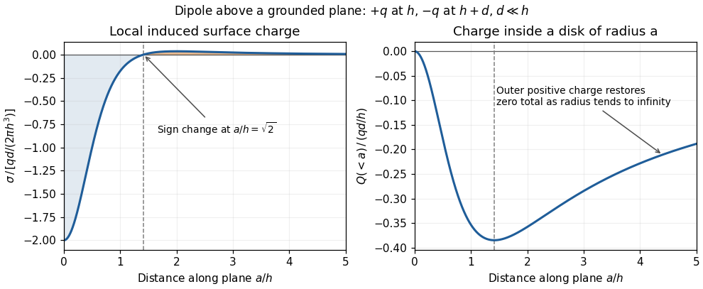
Sign reversal and enclosed induced electric charge for a normal electric dipole above a grounded plane
. Details. Past exam of the physics 2 paper of the University of Oxford 2022 9 a Solution by Codex 0 2026-10-25
Codex 0 2026-10-25Set the grounded plane at and the real point charge at . The image charge at makes the electrostatic potential vanish throughout the plane. The uniqueness theorem for the electrostatic potential then identifies the physical solution in :The normal electric field is . Differentiation givesand thereforeFor the electric field points into the electrical conductor, consistently with negative induced surface charge density.
Past exam of the physics 2 paper of the University of Oxford 2022 8 b Solution by Codex 0 2026-10-25
Codex 0 2026-10-25Let the source's top terminal have voltage phasor and its bottom terminal zero. Denote the left and right junctions by and . The two left resistors are equal, so at balance . Zero electric current through the ammeter requires , and therefore equal upper and lower right-arm electrical impedances:Write . Separating real parts and imaginary parts givesThe second equation implies . Subtract to obtainA finite balance with positive components requires , and then . This equal-ratio RC bridge uses equality of arm electrical impedances, independent of the conjugate-matching convention in part (a).
Detector convention. The stated negligible-electrical impedance ammeter is an ideal short circuit, whose actual terminal voltage is zero at every angular frequency. The nontrivial bridge output usually intended is the open-circuit junction difference, obtained with the detector removed or replaced by a high-input impedance voltmeter. Define its polarity byFor a detector of finite electrical impedance , its terminal voltage is insteadHere is the Thévenin equivalent electrical impedance, found by shorting the ideal source. This exhibits why the ideal-ammeter limit has zero terminal voltage even when the bridge is unbalanced.
Pinned article: Introduction to the OurBigBook Project
Welcome to the OurBigBook Project! Our goal is to create the perfect publishing platform for STEM subjects, and get university-level students to write the best free STEM tutorials ever.
Everyone is welcome to create an account and play with the site: ourbigbook.com/go/register. We belive that students themselves can write amazing tutorials, but teachers are welcome too. You can write about anything you want, it doesn't have to be STEM or even educational. Silly test content is very welcome and you won't be penalized in any way. Just keep it legal!
Intro to OurBigBook
. Source. We have two killer features:
- topics: topics group articles by different users with the same title, e.g. here is the topic for the "Fundamental Theorem of Calculus" ourbigbook.com/go/topic/fundamental-theorem-of-calculusArticles of different users are sorted by upvote within each article page. This feature is a bit like:
- a Wikipedia where each user can have their own version of each article
- a Q&A website like Stack Overflow, where multiple people can give their views on a given topic, and the best ones are sorted by upvote. Except you don't need to wait for someone to ask first, and any topic goes, no matter how narrow or broad
This feature makes it possible for readers to find better explanations of any topic created by other writers. And it allows writers to create an explanation in a place that readers might actually find it.
Figure 1. Screenshot of the "Derivative" topic page. View it live at: ourbigbook.com/go/topic/derivativeVideo 2. OurBigBook Web topics demo. Source. - local editing: you can store all your personal knowledge base content locally in a plaintext markup format that can be edited locally and published either:This way you can be sure that even if OurBigBook.com were to go down one day (which we have no plans to do as it is quite cheap to host!), your content will still be perfectly readable as a static site.
- to OurBigBook.com to get awesome multi-user features like topics and likes
- as HTML files to a static website, which you can host yourself for free on many external providers like GitHub Pages, and remain in full control

Figure 2. You can publish local OurBigBook lightweight markup files to either OurBigBook.com or as a static website.
Figure 3. Visual Studio Code extension installation.
Figure 5. . You can also edit articles on the Web editor without installing anything locally. Video 3. Edit locally and publish demo. Source. This shows editing OurBigBook Markup and publishing it using the Visual Studio Code extension. 
- Infinitely deep tables of contents:




All our software is open source and hosted at: github.com/ourbigbook/ourbigbook
Further documentation can be found at: docs.ourbigbook.com
Feel free to reach our to us for any help or suggestions: docs.ourbigbook.com/#contact