Expand the vector field about the reference trajectory:
Over a sufficiently short interval, the tangent-linear propagator is
Consequently
If has and the perturbation is initially parallel to , its squared Euclidean norm obeys
Positive means instantaneous norm-squared growth, negative decay, and zero no first-order change. The corresponding norm growth rate is , not . These are eigenvalues of the symmetric part governing the chosen error metric, not generally the eigenvalues of the nonsymmetric Jacobian matrix or the long-time Lyapunov exponents. The direction and the reference Jacobian matrix evolve during a finite forecast.
Weather-forecast errors arise from uncertainty in the initial atmospheric state, including measurement noise, incomplete spatial coverage and imperfect data assimilation; from model error, including unresolved clouds, convection and turbulence, approximate physical parameterizations and imperfect boundary forcing; and from discretization, time stepping and roundoff. Sensitive dependence on initial conditions amplifies suitable small errors through nonlinear dynamics, limiting deterministic predictability even with a good model. It is an amplification mechanism rather than a separate observational noise source. Ensemble forecasts sample some initial-state and model uncertainty, but their spread need not represent every systematic error.
Apply the intended, corrected dispersion relation in c. A uniform mean zonal wind gives . Stationarity with therefore requires eastward intrinsic phase speed . With ,
The period determines and . Hence
Figure 1.
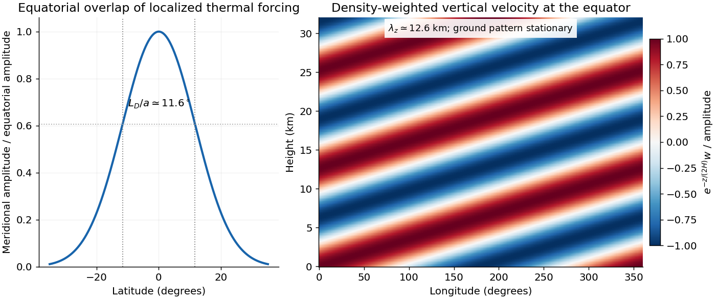
Equatorial trapping and vertical phase of the stationary Martian Kelvin-wave example
. The original calculation uses an eastward intrinsic speed of 20 metres per second. The Gaussian amplitude has a latitude scale of 11.6 degrees; the density-weighted vertical velocity has a vertical wavelength of 12.6 kilometres. The plotted negative vertical wavenumber corresponds to upward intrinsic energy propagation. Details.
A storm within roughly of the equator has substantial projection on the Gaussian mode. There is no sharp latitude cutoff: gives amplitude and the amplitude latitude is about . Forcing outside that core has progressively weaker overlap.
The intrinsic wave is eastward even though its observed ground pattern is stationary; westward advection cancels its phase propagation. Its intrinsic period is about Earth days. The inferred puts it in the short-vertical-wavelength branch, well below the long-wave speed . For upward energy radiation, must be positive, which selects for positive : vertical phase propagation is then downward. Dust absorption supplies thermal forcing with a zonally asymmetric component; the response does not imply that dust itself moves eastward at the intrinsic phase speed.
Southern spring to summer, the warmer perihelion-side dust season, is a reasonable climatological window for such a regional storm. This seasonal inference uses observed dust climatology, not the dispersion relation: the specified wind and wave parameters alone do not determine a unique season, and individual regional storms can occur outside that window.[ref]
Work with the explicitly corrected reduced-pressure system in b. Write and use the complex wave amplitude, taking real parts at the end. The vertical factor satisfies , so the wave equation gives
For a Kelvin wave, continuity, zonal momentum and the buoyancy equation then determine all polarizations:
In particular have amplitude proportional to , whereas pressure has amplitude proportional to . Directly substituting these expressions into vertical momentum gives , verifying both the sign and the dispersion relation.
Meridional momentum is . Since , it integrates to a Gaussian . Thus
The eastward intrinsic branch is selected by decay away from the equator; choosing would make the meridional amplitude grow without bound. Although the squared dispersion relation has both frequency signs, a meridionally trapped Kelvin wave has this one phase-propagation direction.
For short vertical wavelengths, , so , and . The wave is a slowly oscillating, hydrostatic internal gravity wave with strong vertical variation and relatively narrow trapping. Here and ; the buoyancy expression above remains valid.
For long vertical wavelengths, , the exact limiting speed is . To obtain the stated height-controlled limit also requires long horizontal wavelength, . With both and ,
The finite density scale height prevents the hydrostatic phase speed from diverging as . The polarizations tend to , and . Long vertical wavelength alone at fixed large would not justify . In the opposite horizontally short limit the frequency approaches instead. The growth compensates decreasing reference density in wave-energy density; a radiating wave train is a local modal description, not a finite-total-energy eigenfunction over an infinite vertical domain.
First check the printed equations literally. Set and use . Differentiating continuity in time and using horizontal momentum gives
Vertical momentum and buoyancy give . Combining them therefore yields
which differs from the requested equation. The factor two arises when differentiating both and . Keeping variable density in continuity while treating it as constant during that differentiation would be inconsistent.
For the intended anelastic reduced-pressure Kelvin wave, make the explicit correction , while and . Continuity then gives , and vertical momentum gives . Cross differentiation now produces
This proves the advertised equation for the corrected model, without claiming it follows from the incompatible printed set.
A concrete counterexample makes the distinction testable. In nondimensional units , take , and , multiplied by its Gaussian meridional envelope. This satisfies the last boxed wave equation, but substitution into the literal printed-system wave operator gives . No choice of accompanying pressure and horizontal velocity can then make it a solution of all five printed equations. Conversely, the literal operator has vertical factors and dispersion ; its scaling is different from the requested half-scale-height factor.
Take an isothermal hydrostatic reference atmosphere, , and linearize about rest. The horizontal acceleration and pressure-gradient force retain the equatorial Coriolis parameter , with . The traditional approximation retains only its vertical component. Quadratic perturbation advection is neglected. The vertical acceleration is balanced by perturbation buoyancy and pressure gradient after removing the reference hydrostatic balance.
The continuity constraint is the anelastic approximation, , giving . It retains stratification-driven expansion while filtering acoustic density fluctuations. It is therefore not the full compressible continuity equation. Adiabatic displacement in a stably stratified background gives , with the Brunt–Väisälä frequency; upward displacement develops restoring negative buoyancy.
Pressure convention matters. With the entropy-buoyancy equation just described, a consistent reduced-pressure form writes the pressure acceleration as , where . Its vertical term is , not simply . The original source explicitly specifies variable but prints the latter. Those differ by , so the two cannot silently be equated. Parts b and c display the consequence and then solve the explicitly corrected reduced-pressure model that yields the requested wave equation. This is a mathematical inconsistency in the printed set, not missing source material.
A hydrostatic pressure interval contains moles of background gas per area. Its absorbing column is , so for a nadir ray
The assumed Planck-temperature power and dry adiabat give . To first order in optical depth, , and the radiance solution becomes
For a uniform mixing ratio this also evaluates to . Its total optical depth is , so the deficit is .
A pressure-resolved perturbation defines the infrared absorber sensitivity kernel by , with
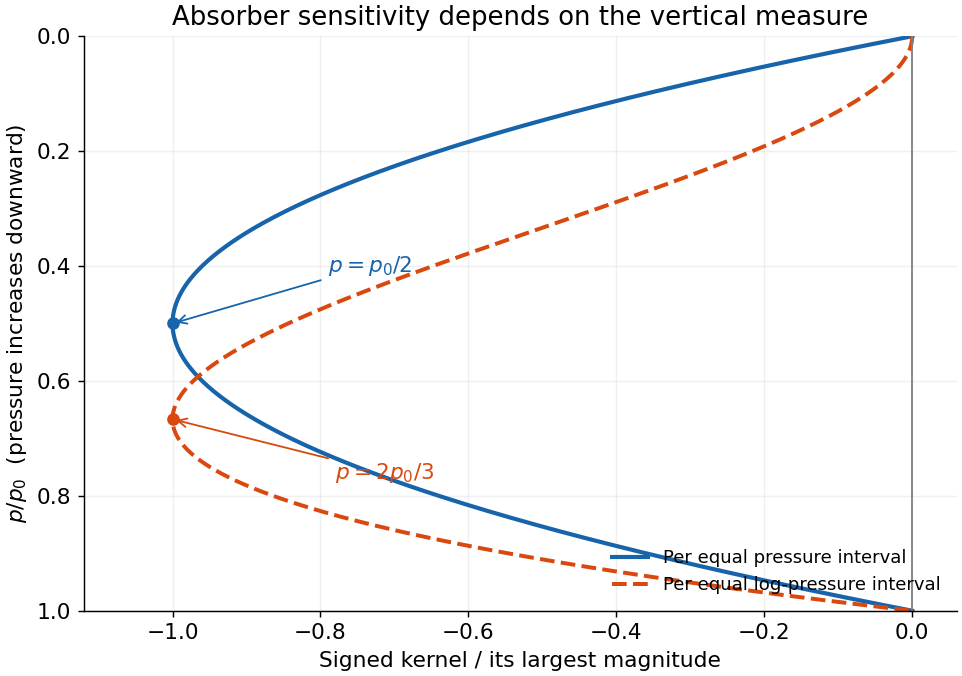
It is zero at the top, negative in the interior, and zero again at the surface. The magnitude is largest where , namely
Sign and coordinate qualification. Literally the maximum of the signed kernel is zero at the endpoints; is its minimum and the maximum of its absolute value. The derivative with respect to a single vertically uniform is the integrated constant and has no pressure location. For equal-width logarithmic pressure perturbations the kernel is instead and its magnitude peaks at . The stated pressure-interval convention is therefore essential.
Figure 1.
Signed infrared absorber sensitivity per pressure interval and per logarithmic pressure interval
. Original normalized kernels vanish at the top and surface. The pressure-interval kernel reaches its most negative value at half the surface pressure; logarithmic-pressure weighting moves the largest-magnitude sensitivity to two thirds of the surface pressure. Details.
The low top-of-atmosphere sensitivity reflects the small pressure-broadened absorption coefficient and small molecular column per there; the low surface sensitivity reflects small thermal contrast. The printed phrase that temperature decreases with pressure reverses the actual stipulated relation: with positive exponent, temperature decreases as pressure decreases upward. The derivation uses the explicit adiabatic formula.
Assume a plane-parallel atmosphere in local thermodynamic equilibrium, negligible infrared scattering, a black surface, and surface temperature equal to the adjacent air temperature. For a specified ray, let be its transmittance from a level to space, increasing from at the surface to one at the top. The formal radiative transfer solution is
Using yields
This expresses absorption and re-emission together: opacity does not simply remove surface radiation without adding atmospheric radiation. An absorber close to a thermally coupled surface has nearly the same Planck function as that surface, so is small. Its emission nearly compensates the surface radiation it absorbs, giving weak radiance sensitivity to near-surface concentration. In an exactly isothermal atmosphere at surface temperature, for every optical depth, a concrete example of complete concentration ambiguity in this thermal measurement. Finite surface emissivity, reflection, scattering or a surface-air temperature discontinuity would require additional terms.
For a unit mass of ideal gas, the first law of thermodynamics in enthalpy form is . A reversible adiabatic displacement has , and the ideal gas law gives . Thus
The atmospheric profile approaches this dry adiabat when convection efficiently mixes potential temperature and there is no condensation or other strong diabatic source. The first law by itself determines a parcel path, not every possible environmental temperature profile; the convective mixing assumption is needed. Hydrostatic balance gives the corresponding height lapse rate .
For rigid linear molecules with translation and rotation active but vibration frozen, the molecular heat capacities are and , hence . Earth is dominated by the diatomic gases nitrogen and oxygen. Mars is dominated by carbon dioxide, which is triatomic but linear and has the same two rotational degrees of freedom. In the rigid-molecule approximation it therefore has the same ratio. The value is not exact for carbon dioxide when its bending vibrations contribute appreciably to heat capacity, and variable heat capacities give a nonconstant dry-adiabatic exponent. Here denotes , not the distinct adiabatic index .
A numerical scale estimate requires a reference ocean density and latitude not specified exactly. Taking , and a representative midlatitude gives
For a small-amplitude interface displacement of scale , gravity drives rapid horizontal acceleration and radiates most of the displacement in inertia-gravity waves. The gravity adjustment time is minutes, much shorter than hours. A weak balanced remnant remains in an unbounded inviscid adjustment problem; energy is carried away by waves, not dissipated merely by geostrophic adjustment.
For , rotational adjustment produces a largely retained interface displacement with a geostrophic current. Wave emission and inertial oscillations accompany the adjustment, but the balanced structure is much more important. To quantify that distinction under an initially resting, linear single-Fourier-component assumption, potential-vorticity conservation gives
This is about for the kilometre scale and for the hundred-kilometre scale. These fractions use as an inverse wavenumber scale, not a full wavelength, and are illustrative rather than unique predictions for an unspecified disturbance or bounded basin.
Let and . The three branches are
For nonzero and , the zero-frequency mode is stationary geostrophic flow, with and zero horizontal divergence. It carries the linear potential-vorticity disturbance. There is no Rossby-wave propagation on a constant- plane; a varying Coriolis parameter would be needed for that.
The other two branches are oppositely phased inertia-gravity waves. Their phase-speed magnitude and radial group velocity are and . When , gravity dominates: and the waves are approximately nondispersive, with both speeds approaching . When , rotation dominates: , the frequency approaches the inertial frequency and the group velocity tends to zero. The large long-wave phase speed is not a large signal speed.
Without rotation the propagating branches become nondispersive gravity waves, , and the stationary branch is a nondivergent vortical velocity disturbance rather than a finite-pressure geostrophic balance. At , the modes reduce to constant interface height and spatially uniform inertial oscillations. The wave branches have zero linear potential-vorticity perturbation; it is the stationary branch that retains the initial potential vorticity.
Write , with small interface displacement and horizontal variation scale . The geostrophic pressure-Coriolis balance gives
Subtracting the uniform reference state and the mass-conserving linear potential-energy term, the perturbation energy densities per unit horizontal area are
Therefore
The internal deformation radius is the distance an internal gravity wave travels in an inverse-Coriolis time. Balanced broad disturbances mainly store available potential energy; balanced fine structures require relatively large kinetic energy. This scale result presupposes small Rossby number ; reducing the length at fixed displacement eventually violates geostrophy. It does not say an initially resting small-scale height perturbation already has that large kinetic energy: such a perturbation undergoes geostrophic adjustment.
Both descriptions are depth-averaged hydrostatic shallow-layer models. In a one-layer free-surface shallow water equations, a homogeneous layer overlies a rigid bottom and its upper surface moves. Surface elevation changes give a restoring acceleration based on full gravity , with external-wave speed . Barotropic coastal storm surges, long surface gravity waves or a basin seiche are examples.
In the rigid-lid reduced gravity model, the movable boundary is a density interface beneath the active upper layer, while the much deeper lower layer remains at rest. The internal interface mode instead has speed and represents, for example, thermocline displacements and an upper-ocean baroclinic eddy. The mathematical shallow-water form is retained with replaced by and with the appropriate interface-depth convention. A freely moving two-layer surface would support both external and internal modes; the rigid lid filters out the fast external mode, and the resting abyss removes its independent dynamics.
Put the rigid lid at , the interface at and . Assume hydrostatic vertical balance and a resting deep layer. Its pressure is , with horizontally uniform . Pressure continuity at the interface then fixes the upper-layer pressure:
Hence its horizontal pressure gradient at fixed is , independent of depth. Taking the horizontal momentum equation and a vertically uniform upper-layer velocity gives
The exact density denominator for upper-layer acceleration is ; the familiar denominator is the small-density-contrast Boussinesq approximation. The restoring pressure is weaker than for a free surface because only the density difference contributes.
The horizontal shallow-layer equations use the vertical component of planetary rotation: . Thus the source's vector notation is interpreted as the projected vector after the traditional approximation. Taking the full magnitude as a midlatitude Coriolis parameter would discard the latitude dependence. Together with layer-volume conservation, the model has .
Denote aerosol optical depth by to distinguish it from cloud optical depth. Retrieve as in d, collocate it with , and estimate an aerosol-to-droplet susceptibility
A regression should control for water content, updraught and cloud regime; aerosol optical depth is not itself a direct measurement of activated nuclei. For an approximately constant over a factor two in aerosol, .
Integrate the supplied cloud albedo susceptibility rather than treating a finite doubling as infinitesimal:
For a small response, . If is the appropriate mean incoming shortwave flux and the fraction of the scene occupied by these clouds, the leading top-of-atmosphere perturbation, positive downward, is
The two transmissions account approximately for the atmosphere above the cloud and may be absorbed into an effective illuminating flux. In the simplest global transparent-overburden estimate . Positive gives increased reflection and negative shortwave forcing, the Twomey effect. Numerical forcing cannot be determined from the given susceptibility alone: it needs baseline albedo, cloud fraction, illumination and an empirically constrained . Humidity swelling, cloud contamination of aerosol retrievals and common meteorological influences can create spurious correlations. Changes in cloud amount, water path or lifetime are additional adjustments, not the fixed-water Twomey term derived here.
In the adiabatic cloud droplet number retrieval, the independently retrieved liquid-water path fixes the geometrical thickness in the adiabatic model:
Define . Since , eliminating gives
Use SI units to obtain in , then divide by for . The sensitivity is substantial: . Thus a numerical retrieval additionally needs the adiabatic condensation coefficient, shape factor and extinction efficiency. A nonadiabatic water profile, mixed phase, horizontal inhomogeneity or a biased water-path retrieval can produce a large number-concentration bias.
Let . The effective droplet radius and shape factor give and , so . If the extinction efficiency is approximately independent of droplet size over the distribution,
For visible wavelengths and droplets large compared with the wavelength, geometrical optics makes a useful approximation. Retaining it as the specified constant, and taking constant over the cloud,
The comes from integrating ; replacing the whole cloud by its cloud-top extinction would incorrectly omit it. The effective-radius relation treats the distribution shape through , without assuming all droplets have the same size. Liquid phase, negligible vertical variation in that shape factor, and negligible departures from the adiabatic water profile are essential assumptions.
Using the adiabatic cloud droplet moments, define and the mean volume radius by . Summing the liquid mass of spherical droplets gives
Therefore, with the shallow-cloud liquid-water content ,
The growth is at fixed number concentration, and the radius scales as at fixed water content. The dimensions are consistent: has units , so has units . The formula is a third-moment radius; a monodisperse distribution is not required. Fixed per volume is the shallow-cloud approximation, not exact conservation of number per parcel volume during an arbitrarily deep expansion.
Below cloud base, an initially unsaturated closed parcel expands as ambient pressure falls. In the absence of heat exchange its temperature falls approximately at the dry adiabatic lapse rate . Its vapour mixing ratio is conserved, but its saturation mixing ratio decreases strongly as it cools. Hence relative humidity rises until the lifting condensation level is reached. The density normally decreases through expansion; the environmental profile determines the parcel's buoyancy and thus whether ascent can continue.
Near saturation, slight atmospheric supersaturation permits suitable cloud condensation nuclei to activate. Köhler theory describes the competition between curvature, which raises equilibrium vapour pressure, and dissolved solute, which lowers it. Cooling generates supersaturation, while condensation onto the new droplets consumes it. Their balance normally keeps in-cloud relative humidity close to, but not identically at, saturation. The activated droplet number depends on the aerosol population and the maximum supersaturation produced by the ascent.
Above cloud base, condensation lowers the vapour content and raises the liquid-water content. The latent heat released partly offsets expansion cooling, so the moist adiabat has a smaller lapse-rate magnitude than the dry one. In a dilute approximation,
A closed adiabatic parcel conserves total water and approximately its moist entropy; retaining condensate makes this a reversible-cloud idealization, rather than a precipitating pseudoadiabat. In a shallow cloud, the saturation-mixing-ratio decrease and slow density variation yield nearly constant condensation per height, so liquid-water content is approximately linear above base. Once activation is complete, assuming nearly fixed droplet number per volume gives increasing droplet size as condensate accumulates. Entrainment, continued activation, collision-coalescence and atmospheric precipitation can all violate that simplified description; they are excluded from the stated retrieval model.
Take a weak line in the radiative sense: the integrated slant optical depth is small wherever absorption materially contributes, not merely a small greenhouse-gas mass mixing ratio. Normalize every local spectral line profile so that , with the line strength independent of pressure and, as stipulated, temperature. Keep a finite Doppler or natural core, or a Voigt profile, so that a pressure-only zero-width core at the top does not invalidate a uniform optical-depth expansion. The line must also be narrow enough to use across it.
To first order,
Thus the detailed normalized line shape drops out, even if its width varies with pressure. Substituting in the deficit in c gives
The neglected term is second order when the relevant squared optical depths are integrable and uniformly small. A very narrow saturated line need not be weak simply because . More generally the displayed first-order integrated limit follows from the finite integrated opacity even if an idealized line centre makes a pointwise expansion nonuniform; a finite physical core is the straightforward sufficient assumption.
For an explicitly perturbative temperature estimate, evaluate the bracket at :
At fixed and radiative conditions, increasing makes every level cooler relative to the surface, enlarging the bracket and the warming. Increasing at fixed has the opposite effect. The limit is isothermal and gives zero line-induced deficit. A change of background molecular mass alone need not change this leading result: for ideal gases with the same active degrees of freedom, and scale together and their ratio is unchanged. Comparing only the height-coordinate lapse rate would miss that the absorber column is naturally a pressure-coordinate quantity.

Pinned article: Introduction to the OurBigBook Project

Welcome to the OurBigBook Project! Our goal is to create the perfect publishing platform for STEM subjects, and get university-level students to write the best free STEM tutorials ever.
Everyone is welcome to create an account and play with the site: ourbigbook.com/go/register. We belive that students themselves can write amazing tutorials, but teachers are welcome too. You can write about anything you want, it doesn't have to be STEM or even educational. Silly test content is very welcome and you won't be penalized in any way. Just keep it legal!
We have two killer features:
  1. topics: topics group articles by different users with the same title, e.g. here is the topic for the "Fundamental Theorem of Calculus" ourbigbook.com/go/topic/fundamental-theorem-of-calculus
    Articles of different users are sorted by upvote within each article page. This feature is a bit like:
    • a Wikipedia where each user can have their own version of each article
    • a Q&A website like Stack Overflow, where multiple people can give their views on a given topic, and the best ones are sorted by upvote. Except you don't need to wait for someone to ask first, and any topic goes, no matter how narrow or broad
    This feature makes it possible for readers to find better explanations of any topic created by other writers. And it allows writers to create an explanation in a place that readers might actually find it.
    Figure 1.
    Screenshot of the "Derivative" topic page
    . View it live at: ourbigbook.com/go/topic/derivative
  2. local editing: you can store all your personal knowledge base content locally in a plaintext markup format that can be edited locally and published either:
    This way you can be sure that even if OurBigBook.com were to go down one day (which we have no plans to do as it is quite cheap to host!), your content will still be perfectly readable as a static site.
    Figure 5. . You can also edit articles on the Web editor without installing anything locally.
    Video 3.
    Edit locally and publish demo
    . Source. This shows editing OurBigBook Markup and publishing it using the Visual Studio Code extension.
  3. https://raw.githubusercontent.com/ourbigbook/ourbigbook-media/master/feature/x/hilbert-space-arrow.png
  4. Infinitely deep tables of contents:
    Figure 6.
    Dynamic article tree with infinitely deep table of contents
    .
    Descendant pages can also show up as toplevel e.g.: ourbigbook.com/cirosantilli/chordate-subclade
All our software is open source and hosted at: github.com/ourbigbook/ourbigbook
Further documentation can be found at: docs.ourbigbook.com
Feel free to reach our to us for any help or suggestions: docs.ourbigbook.com/#contact