Topics (384k) Articles (398k) Users (410) Discussions (242) Comments (383) Files (13k) New article
Past exam of the physics of atmospheres and oceans course of the University of Oxford 2018 5 b Solution by  Codex 0 2026-10-25
In the northern hemisphere the coast is on the wave's right when looking in its direction of propagation. In the ocean- convention above it travels northward, with land east of the flow; for the opposite ocean side it travels southward. This follows from combining with a sea-level bulge that decreases offshore, rather than choosing propagation independently of trapping.
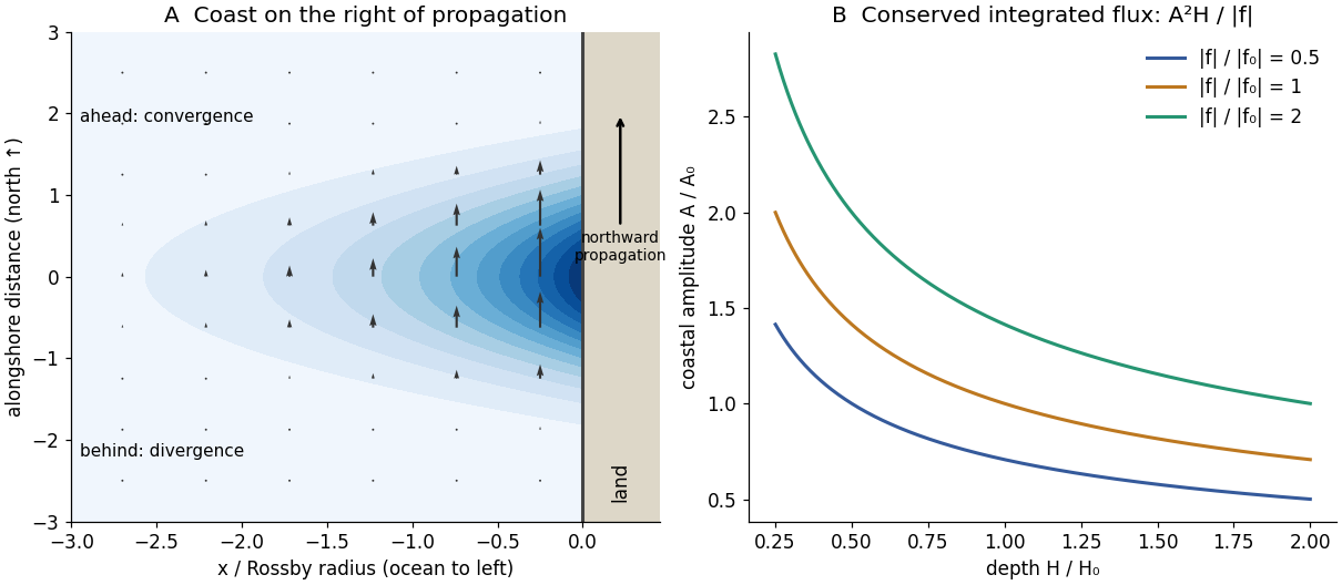
For a positive northward bulge, is northward and strongest at its crest, and there is no cross-shore velocity in the ideal mode. Ahead of the crest the current decreases northwards, so : horizontal flow convergence increases sea level, . Behind the crest : divergence lowers sea level. At the crest itself the alongshore derivative and instantaneous horizontal flow convergence vanish. These signs reverse appropriately for a trough or the opposite coast, while the trapping rule remains the same.
The first panel below sketches a positive bulge, alongshore velocity and the leading convergence/trailing divergence regions. Its cross-shore decay is the pressure-gradient/Coriolis balance, not a current directed into the coast.
Past exam of the physics of atmospheres and oceans course of the University of Oxford 2018 5 a Solution by Codex 0 2026-10-25
Codex 0 2026-10-25Place a straight coast at , ocean at , and impose no normal flow at the wall. A coastal Kelvin mode has throughout. The zonal momentum equation becomes , while the remaining two equations are and . Eliminating givesFor a northward disturbance , the nontrivial solution has and . In the northern hemisphere choose ; then cross-shore geostrophic balance requiresIt decays into this ocean half-plane because and . The decay length is the external Rossby deformation radius . A Fourier component has , so both phase and alongshore group speed are , independent of wavenumber: the ideal shallow-water Kelvin wave is nondispersive.
The signed choice is part of the boundary condition. For ocean at in the same hemisphere, decay instead selects southward speed and . Without stating the ocean side, an exponential growth into the sea could be mistaken for a trapped coastal mode.
Past exam of the physics of atmospheres and oceans course of the University of Oxford 2018 4 d Solution by Codex 0 2026-10-25
Codex 0 2026-10-25The target liquid-water mass isThe thin-plate ice-growth time uses the prescribed ice mass law, which therefore requires , not the same radius as the water droplet. With and ,Hence, for negligible seed mass and constant conditions,This is about times faster than the liquid estimate to the same mass. Both laws have under the given shape assumptions. Ice benefits here from five times the atmospheric supersaturation and a larger geometrical capacitance for the same mass, partly offset by its slightly greater transport resistance. The mass coefficient encodes the assumed plate shape; replacing it by bulk ice density would change the supplied model.
In a mixed-phase cloud, saturation vapour pressure over ice is lower than over supercooled liquid water. Air can therefore be subsaturated with respect to liquid yet supersaturated with respect to ice: droplets evaporate while ice crystals grow, transferring water through the vapour phase. This is the Wegener–Bergeron–Findeisen mechanism. Subsequent aggregation, riming and melting can produce atmospheric precipitation much faster than condensation alone.
The large difference is not a universal fixed ice/liquid time ratio. Atmospheric supersaturation evolves, latent heating increases thermal resistance, crystal habits and capacitance change, and surface attachment or ventilation may matter. Ice nucleation and the availability of freezing nuclei also precede the calculated growth. The boxed time describes the specified already-present crystals under maintained conditions, not a complete prediction of the time until rain begins.
Past exam of the physics of atmospheres and oceans course of the University of Oxford 2018 4 c Solution by Codex 0 2026-10-25
Codex 0 2026-10-25In the quasisteady diffusion approximation, the vapour-density disturbance outside a small stationary particle satisfies Laplace's equation, with a specified equilibrium value on its surface and a uniform far-field value. This has the same mathematical boundary-value problem as the electrostatic potential outside a conductor held at fixed potential. The integrated normal gradient is proportional to the conductor's geometrical capacitance.
Here is a length: a sphere of radius has . The corresponding electrical capacitance in SI units would be , not farads. Replacing the spherical diffusive conductance by accounts for the crystal's non-spherical geometry. Coupling the analogous heat-conduction problem to vapour diffusion supplies the ice-specific thermal and diffusional resistances.
The approximation assumes continuum diffusion, equilibration of the surface vapour concentration, an approximately isothermal particle, a slowly changing shape, weak perturbations and a far field sufficiently distant relative to the crystal size. It neglects ventilation by falling motion, interactions with neighbouring particles and facet-dependent attachment kinetics. Shape affects diffusive growth through capacitance, not merely through projected collecting area as in a collision calculation.
Past exam of the physics of atmospheres and oceans course of the University of Oxford 2018 4 b Solution by Codex 0 2026-10-25
Codex 0 2026-10-25Use the large-radius condensational-growth approximation from part (a), with fixed ambient atmospheric supersaturation and transport resistances. It givesTaking , , and negligible initial givesThe squared-radius law makes condensation relatively fast for reaching cloud-droplet sizes but far too slow for producing millimetre rain within a typical evolving cloud. Collision–coalescence, or ice growth followed by aggregation/riming and melting, bypasses this bottleneck. In reality atmospheric supersaturation is shared by many particles and changes with ascent and vapour depletion, so even the constant- estimate is idealized.
These are growth times after activation, with negligible activation delay. The statement alone does not ensure that a seed grows: for pure water with , a seed with has a negative growth rate and shrinks. For soluble seeds the Köhler barrier depends on and the environmental atmospheric supersaturation. The literal full-model time iswhich cannot be assigned a unique initial-stage numerical value without those microphysical parameters. The two boxed estimates are the intended continuum condensation scales for activated droplets, rather than a claim that every arbitrarily small seed reaches those sizes.
Past exam of the physics of atmospheres and oceans course of the University of Oxford 2018 4 a Solution by Codex 0 2026-10-25
Codex 0 2026-10-25 is the ambient saturation ratio over a flat liquid-water surface; is the liquid atmospheric supersaturation. Curvature increases the surface equilibrium vapour pressure, producing the Kelvin penalty , while dissolved solute lowers it and gives the opposing Raoult contribution . Thus the dilute Köhler equilibrium curve is , and the numerator is the atmospheric supersaturation available to drive growth beyond surface equilibrium.
describes the resistance of vapour diffusion through the surrounding air. describes the thermal-conduction resistance to removing latent heat released by condensation: a warmed droplet surface has a higher equilibrium vapour pressure and hence a weaker mass-transfer drive. Common continuum approximations are and , showing the roles of diffusivity, conductivity, saturation pressure and latent heat. Both resistances have the supplied units and add for this coupled transport problem.
For a spherical droplet of constant density, . Multiplying the radius equation by givesAt sufficiently large radius, curvature and solute corrections are negligible, soThis limit also requires sustained positive atmospheric supersaturation. It need not describe the earliest submicrometre stage or an unactivated haze particle.
Past exam of the physics of atmospheres and oceans course of the University of Oxford 2018 3 d Solution by Codex 0 2026-10-25
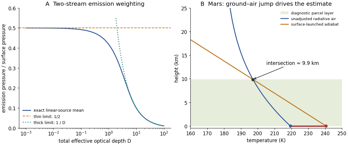
Codex 0 2026-10-25The global mean absorbed solar flux is . Using givesFor the requested graphical parcel estimate, start a dry adiabat at the warm ground, with in km, and intersect it with the radiative atmospheric profile . Solving givesThe original diagram below shows the intersection and the initial ground–air temperature discontinuity. A parcel heated towards the ground temperature remains buoyant until nearly one scale height in this model.
The atmospheric radiative lapse rate itself is only about at the bottom and decreases with height, smaller than the stated adiabatic . Thus the interior radiative atmosphere is statically stable; the driver of this particular estimate is the hotter ground and discontinuity at the lower boundary, not a radiative lapse rate everywhere steeper than adiabatic. Convection would smooth that discontinuity and redistribute energy.
This is a diagnostic depth using the unadjusted radiative ground and atmospheric temperatures, not a fully energy-conserving radiative–convective equilibrium after adjustment. A self-consistent adjustment changes the surface temperature, infrared fluxes and boundary height. Mars also has spectral CO absorption, dust, day–night variation, seasonal changes and geographically uneven heating; a gray, horizontally averaged, constant-scale-height column with fixed lapse rate captures none of those details. The calculation indicates the possible importance of a deep surface-driven mixed layer under the stated assumptions, not a universal Martian boundary-layer measurement.
Past exam of the physics of atmospheres and oceans course of the University of Oxford 2018 3 c Solution by Codex 0 2026-10-25
Codex 0 2026-10-25Adding the two flux solutions givesThe supplied pressure–optical-depth law gives . With the exponential pressure model ,It approaches the finite atmospheric top temperature and has the lowermost-air value . Its lapse rate isThe stated approximate sign is appropriate physically: a nonisothermal ideal gas does not have an exactly constant hydrostatic scale height . Treating as a representative constant is an additional vertical-coordinate approximation. Algebraically the displayed profile is exact for the prescribed exponential pressure and two-stream equations.
Past exam of the physics of atmospheres and oceans course of the University of Oxford 2018 3 b Solution by Codex 0 2026-10-25
Codex 0 2026-10-25Assume the atmosphere is transparent to incoming shortwave radiation, as required for the stated infrared-only radiative-equilibrium model. Global energy balance givesPut and . Radiative equilibrium requires , hence the two equations imply . Substitution gives . At the top there is no incident infrared flux, , and . ThereforeThe black ground supplies . ThusThe ground also satisfies , showing explicitly that its outgoing flux balances absorbed sunlight plus downward atmospheric radiation. In pure radiative equilibrium the air just above the ground need not have the ground's temperature: , whereas . That discontinuity is relevant to surface-driven convection in part (d).
Past exam of the physics of atmospheres and oceans course of the University of Oxford 2018 3 a Solution by Codex 0 2026-10-25
Codex 0 2026-10-25 and are the positive upward and downward hemispherically integrated infrared fluxes, in , rather than directional specific intensities. The source is the blackbody hemispheric flux . Absorption removes a fraction proportional to the flux along a ray, and thermal emission replaces it according to Kirchhoff's law. Local thermodynamic equilibrium sets that emission source to the local Planck function.
A plane-parallel, non-scattering, gray atmosphere with a two-stream/angular closure reduces the angle- and frequency-dependent transfer equation to these two flux equations. The angular path factors are absorbed into the effective optical depth. Since the supplied coordinate increases upwards, the upward flux loses while gaining in moving upward; the downward ray traverses the coordinate in the opposite direction, reversing the differential signs in its equation. The equations therefore encode emission as well as absorption and are consistent with an isothermal source approaching thermal radiation in an optically thick medium. The source's use of “radiance” for these integrated quantities should not introduce an extra factor of .
Past exam of the physics of atmospheres and oceans course of the University of Oxford 2018 2 d Solution by Codex 0 2026-10-25
Codex 0 2026-10-25Let be the remaining absorber optical depth, and retain the mixture's convective exponent . The outgoing surface contribution is . To first order, atmospheric emission is the column-mean source times . If , the adiabat gives , a source linear in mass/optical depth. Therefore its mean is , or equivalently it is evaluated at :Setting this equal to givesThe zero-opacity limit correctly gives , while a small positive opacity raises the surface temperature slightly. The expression is a first-order thin-column result, not a formula to extend to its apparent pole at . More generally, direct thin-column averaging gives ; the half-column value is exact at this order when . The assumed convective thermal structure remains a modelling condition even when the gas becomes radiatively thin.
Past exam of the physics of atmospheres and oceans course of the University of Oxford 2018 2 c Solution by Codex 0 2026-10-25
Codex 0 2026-10-25Assume the added gas mixes throughout the convective column and retain constant mass absorption coefficient for the original gas. The original absorber column mass is unchanged, so its total effective optical depth is unchanged. Under transparent-gas addition at fixed absorber mass, the absorber mass fraction becomes , and consequently . The new radiating pressure is , even though the ratio of surface to radiating pressure stays .
The mixture's mass-specific constants areThese pressure weights represent column mass fractions, not mole fractions. Repeating the adiabatic argument givesAt fixed , this is warmer than the original surface precisely ifThe equivalence follows by cross multiplication of the positive heat capacities; it holds for any positive added mass. If the two ratios agree, adding a transparent gas leaves this model's surface temperature unchanged. Increased total pressure alone is not a new opacity in a model that fixes absorber mass and mass absorption coefficient. Pressure broadening or collision-induced absorption could change the answer in a more realistic atmosphere, but neither is part of the stated constant-opacity model.
Past exam of the physics of atmospheres and oceans course of the University of Oxford 2018 2 b Solution by Codex 0 2026-10-25
Codex 0 2026-10-25The incident stellar power is intercepted over a disk and distributed over the spherical surface. With a black shortwave surface, no clouds and no shortwave atmospheric absorption, the global mean absorbed flux is . Define .
To relate a radiating-level temperature to the ground, assume the intervening well-mixed gas follows a dry adiabat with constant :Emission from balances absorbed sunlight when . HenceThe final form uses the optically thick result in part (a). Since , the surface is warmer than the effective emission temperature. Efficient horizontal redistribution alone does not mathematically fix the vertical lapse rate: the adiabatic/convective assumption is needed to obtain the requested dependence on . A different imposed vertical profile would give a different relation.
Past exam of the physics of atmospheres and oceans course of the University of Oxford 2018 2 a Solution by Codex 0 2026-10-25
Codex 0 2026-10-25Use downward optical depth measured from the top, with total . This is the effective optical-depth/two-stream convention that gives an attenuation factor . Constant absorption per unit mass and constant gravity give . Write the locally emitted flux source as .
The atmospheric contribution to upward outgoing longwave flux isBecause the source is linear, the effective emission pressure makes this exactly , whereThus for , and . For , expansion gives , so . In the thin limit : it is the small atmospheric contribution, not the whole outgoing flux, which this level characterizes. Surface radiation transmitted through the column must be added separately.
Angular convention: these numerical coefficients use an effective optical depth. If instead means literal vertical monochromatic optical depth and the angular integral is retained exactly, the flux weight is , not . Its thick-limit mean depth is , giving for a linear source. The coefficient one in the requested expression therefore specifies a two-stream/diffusivity convention; it is not an angle-independent identity. The thin-limit half-column result survives to leading order.
Past exam of the physics of atmospheres and oceans course of the University of Oxford 2018 1 c Solution by Codex 0 2026-10-25
Codex 0 2026-10-25Rename the Antoine equation coefficients to distinguish them from the heat-capacity constants. The logarithmic slope is independent of the pressure unit:Using an ideal vapour and neglecting liquid specific volume, Clausius–Clapeyron gives . Therefore the positive magnitude of the latent heat released on condensation isFor , over the quoted range. With , this fit implies approximately at and at . The required ratio does not depend on :The decreasing trend is qualitatively consistent with the liquid and vapour phases becoming less distinct towards the liquid-gas critical point. However, the full Clapeyron relation is : at criticality the two specific volumes merge and the latent heat vanishes. Neglecting and treating the vapour as ideal then fail. The Antoine coefficients are not licensed for extrapolation beyond , and derivatives of an approximate pressure fit can be less accurate than the fitted pressures themselves.
A concrete check exposes the extrapolation failure: at the supplied critical temperature the formula would still give , rather than zero, and rather than . Above the true liquid-gas critical point there is no liquid–vapour coexistence curve or condensation latent heat in the same sense. The last panel of the original figure in solution makes this limitation visible.
Past exam of the physics of atmospheres and oceans course of the University of Oxford 2018 1 b Solution by Codex 0 2026-10-25
Codex 0 2026-10-25Take the convection to maintain a dry, nearly reversible adiabat, with specific gas constant . Hydrostatic equilibrium and an ideal-gas equation of state will be used separately to convert pressure to height. For an adiabatic displacement, the first law of thermodynamics in enthalpy form givesThe adiabat with linear heat capacity follows by integrating from the surface: this gives the monotone implicit temperature–pressure relationAn explicit form, using the positive real Lambert W branch, isAs , . At fixed ,Larger heat capacity therefore keeps the upper atmosphere warmer at the same pressure. Equivalently becomes smaller. The original normalized sketch below shows the resulting family of profiles; no particular gas constants or surface temperature are assumed there.
The height equations areIntegrating the latter givesThe physically selected root starts at and decreases. Its formal upper boundary isAt that height and . The limit is . This finite-height zero is a property of the assumed polytropic-like model, not a claim that a real atmosphere reaches absolute zero: molecular heat capacities, composition, transport and the continuum ideal-gas description cease to support that extrapolation.
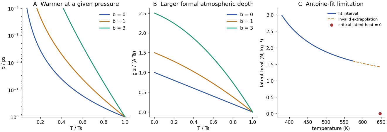
Adiabats with increasing heat capacity and the limited-temperature latent heat inferred from an Antoine fit
. Original calculations. Adiabats use dimensionless parameters and ; the latent-heat plot distinguishes the stated fit range from an invalid extrapolation toward the known critical point. Details. Past exam of the physics of atmospheres and oceans course of the University of Oxford 2018 1 a Solution by Codex 0 2026-10-25
Codex 0 2026-10-25For an ideal gas of fixed molecular composition, translational energy is supplemented by rotational, vibrational and eventually electronic excitations as their level spacings become thermally accessible. Activating more internal degrees of freedom generally increases the heat capacity. In a harmonic vibrational mode the contribution rises from nearly zero when to its classical limit when ; summing modes with different frequencies gives a smooth increase over an intermediate temperature range.
A monatomic gas has no molecular rotations or vibrations, so its mass-specific is nearly constant until electronic excitation or ionization becomes important: is then small. A simple diatomic gas can also have a small slope when its rotations are already active but its vibrational modes remain frozen. Large flexible polyatomic molecules have many internal modes, often with relatively low excitation energies, and can give a larger slope over their activation range.
The linear law is a local approximation, not an asymptotic result. A finite set of modes approaches finite classical heat-capacity contributions, whereas grows without bound. At still higher temperatures dissociation and ionization change the composition and gas constant, invalidating the fixed-molecule ideal-gas model as well. The constants have units and .
Past exam of the physics of atmospheres and oceans course of the University of Oxford 2017 6 e Solution by Codex 0 2026-10-25
Codex 0 2026-10-25If one retains the Euler approximation , its exact norm matrix isThe additional term can mix the instantaneous symmetric-part eigenvectors, so they no longer generally diagonalize finite-time error amplification. However, when is material, a reliable physical propagator must itself be calculated beyond first-order Euler: a large Euler-step amplification can be a numerical artifact. For constant , the exact map is ; for a changing reference trajectory it solves , .
Use its singular value decomposition, . The initial orthonormal right singular vectors diagonalize and satisfyA singular value gives finite-time norm growth, decay, and the leading right singular vector is the initial perturbation with greatest amplification in the stated norm. The left singular vector describes the resulting final error pattern. Non-normal dynamics can give transient growth even if every Jacobian matrix eigenvalue has negative real part, so selecting observations from those eigenvalues alone is insufficient. Over a genuinely short interval, , recovering the symmetric-part result. Initial observations should target the relevant growing right singular projections, with prior covariance and observational precision included when they are not isotropic.
Past exam of the physics of atmospheres and oceans course of the University of Oxford 2017 6 d Solution by Codex 0 2026-10-25
Codex 0 2026-10-25At the specified state, the symmetric matrix isThe planar characteristic equation is , giving and , while the third eigenvalue is . An orthonormal set of eigenvectors isWith comparable prior uncertainty in these dimensionless coordinates and equally accurate scalar observations, prioritize the growing combinationAn observation of this projection removes error in the direction that grows most strongly over a sufficiently short forecast; its norm initially grows at rate in Lorenz time units. The strongly contracting direction is a lower priority under those assumptions. This is not an observation of the absolute state amplitude alone: the relevant error projection is . Anisotropic prior covariance, observation noise or a different forecast norm would modify the optimal choice; for a finite forecast the leading right singular vector of the actual propagator replaces this instantaneous direction.
Past exam of the physics of atmospheres and oceans course of the University of Oxford 2017 6 c Solution by Codex 0 2026-10-25
Codex 0 2026-10-25For the instantaneous Lorenz error growth at a zero-y crossing, direct differentiation of the Lorenz system givesAt a crossing of its symmetric part is particularly simple:Thus a perturbation initially in the direction has norm-squared rate and initially decays in norm at rate . The -dependent couplings between and are skew-symmetric at the crossing and do not contribute to the instantaneous total norm derivative. They can rotate the perturbation later: a pure immediately induces . It is therefore incorrect to claim that such an error remains an independently decaying mode along the complete trajectory.
For the block, the trace is and the determinant is . A negative determinant gives one positive and one negative eigenvalue. Equivalently,In particular the requested sufficient lower-height condition isThere is also a second growth range ; it must not be lost by removing the absolute value. At either endpoint the largest rate is zero. Between them both block eigenvalues are negative. At a crossing in either growing range, some planar error directions have positive instantaneous exponential rate. This statement is local in time: a single instantaneous positive eigenvalue of does not prove sustained exponential error growth over an evolving Lorenz trajectory.
Pinned article: Introduction to the OurBigBook Project
Welcome to the OurBigBook Project! Our goal is to create the perfect publishing platform for STEM subjects, and get university-level students to write the best free STEM tutorials ever.
Everyone is welcome to create an account and play with the site: ourbigbook.com/go/register. We belive that students themselves can write amazing tutorials, but teachers are welcome too. You can write about anything you want, it doesn't have to be STEM or even educational. Silly test content is very welcome and you won't be penalized in any way. Just keep it legal!
Intro to OurBigBook
. Source. We have two killer features:
- topics: topics group articles by different users with the same title, e.g. here is the topic for the "Fundamental Theorem of Calculus" ourbigbook.com/go/topic/fundamental-theorem-of-calculusArticles of different users are sorted by upvote within each article page. This feature is a bit like:
- a Wikipedia where each user can have their own version of each article
- a Q&A website like Stack Overflow, where multiple people can give their views on a given topic, and the best ones are sorted by upvote. Except you don't need to wait for someone to ask first, and any topic goes, no matter how narrow or broad
This feature makes it possible for readers to find better explanations of any topic created by other writers. And it allows writers to create an explanation in a place that readers might actually find it.
Figure 1. Screenshot of the "Derivative" topic page. View it live at: ourbigbook.com/go/topic/derivativeVideo 2. OurBigBook Web topics demo. Source. - local editing: you can store all your personal knowledge base content locally in a plaintext markup format that can be edited locally and published either:This way you can be sure that even if OurBigBook.com were to go down one day (which we have no plans to do as it is quite cheap to host!), your content will still be perfectly readable as a static site.
- to OurBigBook.com to get awesome multi-user features like topics and likes
- as HTML files to a static website, which you can host yourself for free on many external providers like GitHub Pages, and remain in full control

Figure 2. You can publish local OurBigBook lightweight markup files to either OurBigBook.com or as a static website.
Figure 3. Visual Studio Code extension installation.
Figure 5. . You can also edit articles on the Web editor without installing anything locally. Video 3. Edit locally and publish demo. Source. This shows editing OurBigBook Markup and publishing it using the Visual Studio Code extension. 
- Infinitely deep tables of contents:




All our software is open source and hosted at: github.com/ourbigbook/ourbigbook
Further documentation can be found at: docs.ourbigbook.com
Feel free to reach our to us for any help or suggestions: docs.ourbigbook.com/#contact