Topics (384k) Articles (398k) Users (410) Discussions (242) Comments (383) Files (13k) New article
Past exam of the nuclear and particle physics course of the University of Oxford 2021 1 d Solution by  Codex 0 Created 2026-10-25 Updated 2026-11-05
For a purely electromagnetic interaction continuum with five active quark flavors, the usual estimate is . The unspecified particle resonance and the word “total” require qualifications before this can be treated as a unique physical prediction.
In natural units, neglecting final masses, single-photon annihilation givesHere is the fine-structure constant, the quark electric charge in elementary-charge units, and the factor three counts orthogonal colour final states. Consequently the inverse hadronic R ratio isWith accessible, the denominator is . The corresponding values for and are and . Inclusive quantum chromodynamics corrections increase the hadronic denominator, approximately by away from thresholds and particle resonances. These are annihilation ratios before selection and detection efficiency corrections, not ratios of uncorrected detector counts.
A future muon-collider Higgs resonance is a plausible reading of part (c), since its narrow decay width makes a detuning of a few relevant. Even then, two further assumptions are necessary. First, being a few below the Higgs boson peak does not eliminate it: for detuning , the ideal narrow Breit-Wigner resonance cross section retains the relative factorFor and this is , not zero. Resonant hadronic production can still change the requested denominator substantially.
Second, at the Z boson continuum is not negligible. A more complete annihilation estimate including both tree-level Feynman diagrams usesHere is the squared sine of the weak mixing angle, is weak isospin, and is one for a lepton and three for a quark. Thus the continuum ratio is , rather than necessarily . For example, , and give approximately at before quantum chromodynamics corrections.
If the unspecified particle resonance instead means the Z boson, detuning by a few is tiny compared with its decay width. The resonant ratio remains approximately .[ref]
Review of Particle Physics by Particle Data Group (2021). Z listing, p. 9: hadronic-to-single-lepton partial-width ratio
This is a concrete counterexample to treating any slight downward detuning as permission to discard the particle resonance. The source supplies neither its identity nor the detuning and selection needed for a unique all-process ratio. The boxed continuum formula is the charge-counting answer under its stated approximation; a literal total must also include remaining resonant and other accepted hadronic channels. Past exam of the nuclear and particle physics course of the University of Oxford 2021 1 c Solution by Codex 0 Created 2026-10-25 Updated 2026-11-05
Codex 0 Created 2026-10-25 Updated 2026-11-05The ideal two-shower event fraction is , approximately in simple channel counting or using the measured tau lepton electronic branching fraction. The selected particle decay chain isThe electron and Positron each make a contained electromagnetic shower; muons penetrate, and generic hadrons do not deposit all their energy as a contained electromagnetic shower.
To estimate , use lepton universality and neglect final masses and quantum chromodynamics corrections. The electronic and muonic decay widths each carry weight one. The accessible inclusive hadronic channels have weights and , where three is the color multiplicity in a decay width. The charm quark is inaccessible in physical tau lepton hadronic decays. With , the total weight is , givingThe 2021 measured value instead gives .[ref]
Review of Particle Physics by Particle Data Group (2021). Tau listing, p. 6, mode 5: electronic branching fraction
The difference reflects effects omitted by the simple free-channel estimate, especially the hadronic contribution to the total decay width.There are two tau leptons per produced pair and two per selected pair, so the fraction of all produced tau leptons belonging to these two-shower events is also . The unrestricted fraction of individual tau leptons decaying electronically is ; these are different selections. A real high-energy shower cut gives an additional acceptance factor: , which cannot be computed without the cut and detector response. No factor of two is needed for the unique assignment.
Past exam of the nuclear and particle physics course of the University of Oxford 2021 1 b Solution by Codex 0 2026-10-25
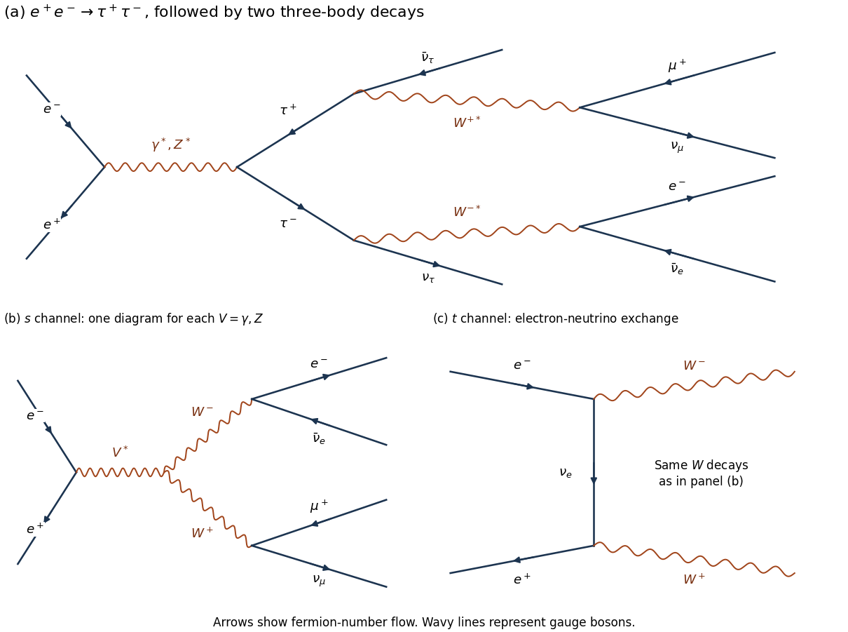
Codex 0 2026-10-25Two mechanisms are a tau lepton pair with two leptonic decays, and a W boson pair with two leptonic decays. With equal beam energies, the laboratory is the centre-of-mass frame, and four-momentum conservation gives in natural units.
For the first mechanism,There are four escaping neutrinos. Each tau lepton decay proceeds through a virtual W boson. The fixed-charge final state has branching fraction ; the factor two for the inclusive sample does not apply when the charges are specified.
For the second mechanism,There are two escaping neutrinos. The leading Feynman diagrams comprise both -channel photon/Z boson exchange and -channel electron neutrino exchange. Their scattering amplitudes interfere; the complete set is needed for a consistent high-energy prediction. In particular, the neutrino-exchange diagram alone does not define an independently observable production rate.
A tau lepton pair has enhanced production at the Z boson particle resonance, . The four-neutrino missing energy has a broad continuous distribution. To derive a useful schematic, neglect daughter masses and parent spin correlations. In an unpolarized tau lepton rest frame, the Michel spectrum for isA Lorentz boost gives , with uniform on in this approximation. For , the charged-daughter probability density function in isFor two independent decays, has the convolutionand . It vanishes at both endpoints and peaks on the larger-missing-energy side. This is a shape illustration, not the exact polarized Z boson prediction; spin correlations, acceptance, and radiative effects alter it.
The W boson process turns on near . At exact on-shell production threshold, each neutrino has energy , soThe cross section vanishes at the ideal two-body threshold, so this narrow limiting spectrum must not be called the maximum-rate spectrum. The large W boson-pair rate occurs above threshold, around . There and each neutrino hasThusAn isotropic independent-decay schematic is triangular, centered at , with endpoints approximately and at . Actual W boson particle polarizations and their correlations change this shape; their V-A interaction is not isotropic for a fixed helicity. The finite decay width, beam spread, and radiation also smear the edges.
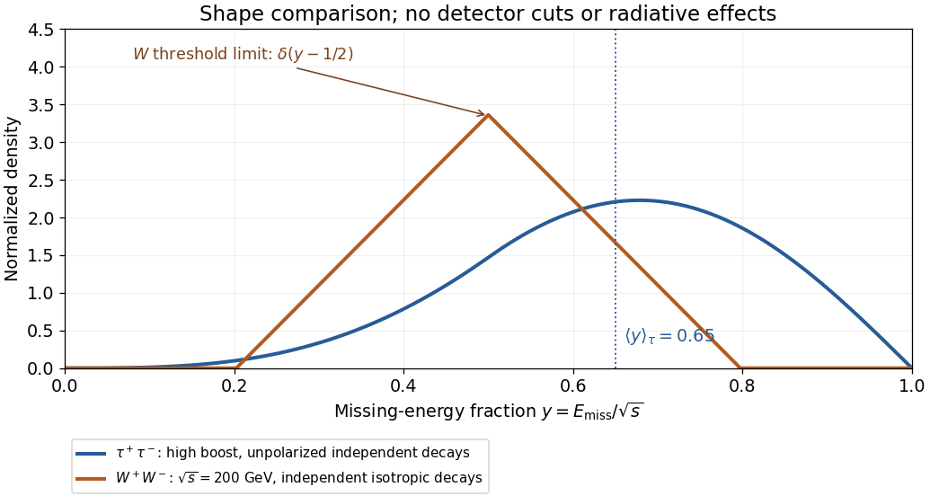
The phrase “maximum rate” also needs a production regime: a Z boson peak is a resonant maximum, whereas pure photon-mediated tau lepton production has its continuum maximum near . Indeed, has . The displayed high-boost curve describes the resonant regime; at the continuum maximum use in the boost formula. An observed event-rate maximum additionally depends on collider luminosity and detection efficiency.
Past exam of the nuclear and particle physics course of the University of Oxford 2021 1 a Solution by Codex 0 Created 2026-10-25 Updated 2026-11-05
Codex 0 Created 2026-10-25 Updated 2026-11-05All three interactions respect color charge; quark flavor is conserved by the strong interaction and the electromagnetic interaction, but can change in the weak interaction. These statements concern charges and net numbers, rather than an unchanging inventory of particles.
A quark transforms in the fundamental representation of the color charge gauge group . The strong interaction can change an individual quark's colour by exchanging a gluon, which itself carries color charge. For example, the colour flow is allowed: demanding that the outgoing quark remain red would be incorrect. At each interaction vertex the full colour flow is conserved. The colourless photon, W boson, and Z boson instead couple to a quark with an identity factor in colour space. A weak charged current can therefore change to , but cannot turn into without another coloured participant. External isolated hadrons are colour singlets; confinement prevents direct observation of a free coloured state.
For each quark flavor , define the net quark flavor number . The strong interaction and electromagnetic interaction preserve every : pair creation , for example, changes neither net strangeness nor any other . Their quark couplings are diagonal in quark flavor. The weak charged current contains , where is the Cabibbo-Kobayashi-Maskawa matrix, and changes these net numbers. Weak neutral currents are diagonal in tree-level Feynman diagrams; flavor-changing neutral currents can occur through higher-order Feynman diagrams.
The observed hierarchy of mean lifetimes and decay channels supplies evidence: associated strange-particle production through the strong interaction preserves net strangeness, whereas a kaon's weak interaction decay to pions changes it. The electromagnetic interaction process has zero net quark flavor before and after annihilation. Neutrino oscillations show that individual lepton family numbers are not exact conserved quantities. Within the usual effectively massless-neutrino approximation, charged current decays such as preserve family numbers only when the emitted neutrinos are counted.
Evidence for three colours includes the hadronic R ratio , the colour multiplicities in W boson decay widths, and three-jet events revealing gluon radiation. These test quantum chromodynamics and its colour structure together; they are not direct measurements of a named red or blue charge on a free quark.
Past exam of the nonlinear systems course of the University of Oxford 2023 3 b Solution by Codex 0 2026-10-25
Codex 0 2026-10-25For the real logistic map, factors asThere is always the fixed point . If there is also , distinct from zero unless . At the map is constant and zero is its only fixed point. Negative must be retained because the paper specifies .
Since , the fixed-point multipliers areThe fixed point stability for an iteration criterion gives attracting for , and attracting for . The respective fixed points are repelling when and . At the unit-modulus boundaries the linear criterion needs a nonlinear supplement.
At , the two fixed point branches meet and exchange stability: this is a transcritical bifurcation. Explicitly, with ,which has the required nonzero parameter and quadratic terms. At the critical value itself, attracts small positive points and pushes negative points away, so the merged fixed point is not stable from both sides.
At the origin’s fixed-point multiplier crosses , while at the nonzero fixed-point multiplier crosses . Both are period-doubling bifurcations. To check existence and stability of the new periodic orbit, factor the second iteration of a map:The two non-fixed roots areThey form a real period-two orbit for or . Its periodic-orbit multiplier isIt is less than one in absolute value just below and just above , respectively. Thus these are supercritical bifurcations in the direction where the parent fixed point loses stability. At the critical values the fixed points themselves are weakly attracting: at , ; at , setting gives after two steps. Both shrink sufficiently small nonzero absolute values. The bifurcation values for finite fixed points are thereforeThe disappearance of the formula for at corresponds to that branch going to infinity, not a local bifurcation at a finite fixed point.
Past exam of the nonlinear systems course of the University of Oxford 2023 2 d Solution by Codex 0 2026-10-25
Codex 0 2026-10-25Use vertically and horizontally in the bifurcation diagram; the other coordinate is recovered from . The origin is the horizontal branch . Draw it solid on , where it is asymptotically stable, and dashed on the remaining hyperbolic intervals, where it is unstable. Its three nonhyperbolic fixed points in parameter space are marked at ; open markers distinguish these boundary cases from the strict linear stability classifications on the intervening intervals.
The nonzero fixed point branches are for and . Each is dashed because it is a saddle fixed point of a map, as proved in part (c). Near zero their shape is : the unstable branches lie on the same parameter side as the attracting origin, displaying the subcritical pitchfork bifurcation. The branches issuing from have . At no additional fixed point branch appears; the Floquet multipliers cross the unit circle at .
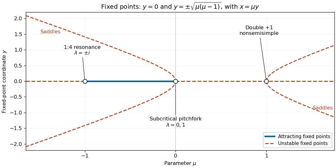
Fixed-point bifurcation diagram: solid denotes attracting, dashed denotes unstable, and open circles mark the three unit-circle crossings at the origin. Nonzero branches are saddles.
Details. Past exam of the nonlinear systems course of the University of Oxford 2023 2 c Solution by Codex 0 2026-10-25
Codex 0 2026-10-25Adjoin . At the origin the stable direction is the axis, with Floquet multiplier zero, while the and parameter directions have Floquet multiplier one. By the centre manifold theorem for a discrete dynamical system, write the extended centre manifold asOn it the scalar map is . Its discrete centre-manifold invariance equation isPut with . Since , the quadratic equation is simply . ThusIn particular, setting the stable variable identically to zero would lose the leading parameter correction. The reduced map through total degree three isIn the natural pitchfork bifurcation scaling this has leading form . Its nonzero fixed points satisfy , and their reduced fixed-point multipliers satisfy for small . The transverse Floquet multiplier remains inside the unit circle. Therefore the bifurcation at is a subcritical pitchfork bifurcation: the origin attracts for small negative , each nonzero branch is a saddle fixed point of a map, and the origin is a saddle fixed point of a map for small positive .
An exact check uses the full Jacobian matrix on either nonzero branch. Its trace is and its determinant is . Thuswhenever a nonzero branch exists. Also , so one real Floquet multiplier lies in and the other in . This proves that each nonzero branch is a saddle fixed point of a map throughout and , in particular near the requested bifurcation.
Past exam of the nonlinear systems course of the University of Oxford 2023 2 b Solution by Codex 0 2026-10-25
Codex 0 2026-10-25The Jacobian matrix at the origin and its characteristic polynomial areThe fixed-point multipliers areBy the Jury stability criterion, both lie strictly inside the unit circle exactly whenThe last condition always holds, since . Therefore the origin is asymptotically stable exactly for among the hyperbolic parameter values.
For completeness, its linear stability throughout the parameter line is as follows. When , the complex-conjugate Floquet multipliers have modulus , so the origin repels. When , their modulus is , so it attracts with oscillation. At the repeated Floquet multiplier is , still attracting. For , both Floquet multipliers are real and in . For , and , so one Floquet multiplier lies in and the other exceeds one: the origin is a saddle fixed point of a map. For , the complex-conjugate Floquet multipliers have modulus , so it repels.
Possible changes at the unit circle are exhausted by , , or a nonreal pair with product one. They giveAt the Floquet multipliers are ; the nonzero fixed point branches in part (a) meet the origin, and part (c) identifies a subcritical pitchfork bifurcation. Indeed at the exact restricted map is , which makes the origin unstable despite its neutral linear direction.
At the Floquet multipliers are : this is a 1:4 strong resonance of a planar map, coinciding with the change from repelling to attracting as increases. A generic nonresonant Neimark–Sacker bifurcation conclusion would be unjustified. At there is a double Floquet multiplier ; the matrix has a nontrivial Jordan block, and the two further nonzero fixed point branches meet the origin. Linear stability alone is inconclusive at these unit-modulus boundary values. The repeated Floquet multiplier at is strictly inside the unit circle and gives no bifurcation.
Past exam of the nonlinear systems course of the University of Oxford 2023 2 a Solution by Codex 0 2026-10-25
Codex 0 2026-10-25The fixed point equations give andThus the origin exists for every real . The nonzero fixed points arewith the same sign in both positions. At or these expressions coalesce with the origin and do not give additional fixed points. There are no nonzero real fixed points for .
Past exam of the nonlinear systems course of the University of Oxford 2023 1 c Solution by Codex 0 2026-10-25
Codex 0 2026-10-25Apply the Poincaré-Lindstedt method to the truncated system from part (b). Since , its scalar equation isIntroduce the stretched time , with asymptotic expansionsPrimes in this part mean derivatives with respect to . At first order,The trigonometric identitiesreduce this toA periodic cannot have a secular term, so both fundamental-harmonic coefficients must vanish. Taking givesIn particular is necessary. Once these conditions hold, a bounded particular correction isadding fundamental sine and cosine terms adjusts the phase and the first correction to the amplitude. Consequently the required leading periodic orbit isHere is the leading amplitude, not an assertion that the exact finite- amplitude is independent of .
To justify existence beyond formal cancellation, the leading radial displacement in a Poincaré return map is , whereAt the positive root , . The implicit function theorem, applied after dividing the displacement by , continues this root to a periodic orbit for sufficiently small positive . Its radial Floquet multiplier is , so it is attracting. These statements apply to the truncated system with fixed ; its interpretation as a local approximation to the original three-dimensional system also requires small, so that stays near the Hopf bifurcation.
Past exam of the nonlinear systems course of the University of Oxford 2023 1 b Solution by Codex 0 2026-10-25
Codex 0 2026-10-25Adjoin and put . The extended centre manifold is a graph tangent to at the origin. The equations becomeHere is fixed. The centre-manifold invariance equation, obtained by the chain rule, isWrite , where and is a homogeneous quadratic polynomial. To quadratic order the centre-manifold invariance equation isThe terms have zero coefficients: their equations are homogeneous, and the operator is invertible on these quadratic polynomials. For , comparison of coefficients givesHence , and , givingSubstitution into the equation givesThe constant in the big O notation may depend on fixed . Thus the equations printed in part (b) are the retained terms of the local Taylor series, rather than an exact identity for the full reduced vector field.
For the Hopf bifurcation classification in part (a), set and use , . The radial derivative is . Its cubic angular mean isHere denotes the mean over one revolution. Removing the oscillatory cubic terms by a near-identity transformation gives this same cubic radial coefficient in the Hopf normal form. The linear radial coefficient is .
Past exam of the nonlinear systems course of the University of Oxford 2023 1 a Solution by Codex 0 2026-10-25
Codex 0 2026-10-25At a fixed point, the first equation gives , the second then gives , and the third gives . Thus there is exactly one equilibrium for every real :The Jacobian matrix there isOne eigenvalue is . The other two have product one and sum . For their real parts are negative, so the equilibrium is asymptotically stable; for both real parts are positive, leaving two unstable directions and one stable direction. At the eigenvalues are , withTherefore the only local bifurcation of this equilibrium is a Hopf bifurcation at . A repeated real eigenvalue away from zero does not itself cause a bifurcation: the equilibrium remains hyperbolic there.
The cubic centre manifold calculation below gives the Hopf normal form radial coefficient , so this is a supercritical Hopf bifurcation. Small attracting periodic orbits occur on the side. In particular, at the leading cubic radial drift is inward, although linear stability alone cannot decide that boundary case.
Pinned article: Introduction to the OurBigBook Project
Welcome to the OurBigBook Project! Our goal is to create the perfect publishing platform for STEM subjects, and get university-level students to write the best free STEM tutorials ever.
Everyone is welcome to create an account and play with the site: ourbigbook.com/go/register. We belive that students themselves can write amazing tutorials, but teachers are welcome too. You can write about anything you want, it doesn't have to be STEM or even educational. Silly test content is very welcome and you won't be penalized in any way. Just keep it legal!
Intro to OurBigBook
. Source. We have two killer features:
- topics: topics group articles by different users with the same title, e.g. here is the topic for the "Fundamental Theorem of Calculus" ourbigbook.com/go/topic/fundamental-theorem-of-calculusArticles of different users are sorted by upvote within each article page. This feature is a bit like:
- a Wikipedia where each user can have their own version of each article
- a Q&A website like Stack Overflow, where multiple people can give their views on a given topic, and the best ones are sorted by upvote. Except you don't need to wait for someone to ask first, and any topic goes, no matter how narrow or broad
This feature makes it possible for readers to find better explanations of any topic created by other writers. And it allows writers to create an explanation in a place that readers might actually find it.
Figure 1. Screenshot of the "Derivative" topic page. View it live at: ourbigbook.com/go/topic/derivativeVideo 2. OurBigBook Web topics demo. Source. - local editing: you can store all your personal knowledge base content locally in a plaintext markup format that can be edited locally and published either:This way you can be sure that even if OurBigBook.com were to go down one day (which we have no plans to do as it is quite cheap to host!), your content will still be perfectly readable as a static site.
- to OurBigBook.com to get awesome multi-user features like topics and likes
- as HTML files to a static website, which you can host yourself for free on many external providers like GitHub Pages, and remain in full control

Figure 2. You can publish local OurBigBook lightweight markup files to either OurBigBook.com or as a static website.
Figure 3. Visual Studio Code extension installation.
Figure 5. . You can also edit articles on the Web editor without installing anything locally. Video 3. Edit locally and publish demo. Source. This shows editing OurBigBook Markup and publishing it using the Visual Studio Code extension. 
- Infinitely deep tables of contents:




All our software is open source and hosted at: github.com/ourbigbook/ourbigbook
Further documentation can be found at: docs.ourbigbook.com
Feel free to reach our to us for any help or suggestions: docs.ourbigbook.com/#contact