Topics (384k) Articles (398k) Users (410) Discussions (242) Comments (383) Files (13k) New article
Past exam of the further quantum theory course of the University of Oxford 2023 2 e Solution by  Codex 0 2026-10-25
For , the Hamiltonian operator is nonnegative: its quadratic form is . Thus it has no negative-energy bound states. A nonnegative-energy exterior wavefunction cannot be square integrable unless it vanishes identically, so there are no other bound states either.
For , set . The even equation is the zero of . Since , and , the intermediate value theorem and strict monotonicity give exactly one positive equation root.
The odd equation is the zero of . Here , , , and . If , strict concavity makes for every . If , initially increases, has exactly one maximum, and then decreases through zero exactly once. This proves the bound-state count of an attractive symmetric double-delta potential:At the threshold , the odd zero-energy solution is proportional to inside and to outside. It is bounded but not a square-integrable function, so it is a zero-energy scattering resonance rather than a second bound state. Each negative-energy bound state is either even or odd by nondegeneracy of one-dimensional bound states; the two branches above exhaust the count.
Past exam of the further quantum theory course of the University of Oxford 2023 2 d Solution by Codex 0 2026-10-25
Codex 0 2026-10-25Continue the transmission amplitude to complex wavenumber with , equivalently complex momentum . Then . In the left exterior region the term grows at negative infinity and the term decays; in the right exterior region the term grows and the term decays. A bound state thus requires , with nonzero . The transfer matrix relation gives . Equivalently, a zero of the incoming coefficient is a bound-state pole of , whose numerator is nonzero at .
The denominator found in part (c) givesFactorization produces two branches. To identify their parity, use an even interior wavefunction or an odd interior wavefunction for , joined to a decaying exterior wavefunction at . Continuity and the derivative jump give, respectively,Rearrangement gives the implicit energy eigenvalue equationsOnly strictly positive equation roots are retained. With , the even equation root lies above and the odd equation root, when it exists, lies below , so the even bound state has lower energy. The formal zero equation root in the odd equation does not itself establish a normalizable wavefunction.
Past exam of the further quantum theory course of the University of Oxford 2023 2 c Solution by Codex 0 2026-10-25
Codex 0 2026-10-25Assume and put , , and . At a delta potential located at , integration of the Schrödinger equation gives the matching conditionsWriting the adjacent plane wave coefficients as and givesSolving these two linear equations yields the transfer matrix of a delta potential:For the symmetric double-delta potential, use separate plane wave pairs in , , and . Successive matching gives between the two exterior pairs. For real , multiplication givesThe determinant identity reads . Left incidence means , whenceHere the first relation also follows from . Therefore the requested transmission probability and quantum reflection probability, as functions of the printed momentum , areThey obey . As checks, gives , and the coincident limit gives , the answer for a single delta potential of strength .
Past exam of the further quantum theory course of the University of Oxford 2023 2 b Solution by Codex 0 2026-10-25
Codex 0 2026-10-25For a real potential energy and a stationary state, the probability current isThe time-independent Schrödinger equation gives , so . In an exterior plane wave superposition, interference terms contribute no current andConsequently for every choice of incoming amplitudes. If , this says for every complex vector . Since is Hermitian, vanishing of its quadratic form implies that the matrix itself vanishes. ThereforeThe second identity follows by choosing . Since is a square matrix, the first also implies , proving unitarity. A real delta potential preserves this proof: continuity of and the real derivative jump make the current continuous across the interaction point.
Past exam of the further quantum theory course of the University of Oxford 2023 2 a Solution by Codex 0 2026-10-25
Codex 0 2026-10-25For , put and . Outside the support of the potential energy, a generalized eigenfunction of the Hamiltonian operator has the plane wave formHere denotes the support radius, to distinguish it from the quantum reflection probability . The momenta are and the velocities are . Thus describe incoming scattering channels from the left and right, and describe outgoing scattering channels towards the left and right. These energy eigenfunctions are not square-integrable functions; normalizable incoming wave packets are formed by superposition over energy, and their passage through the interaction region gives the physical quantum scattering experiment.
For incidence from the left, normalize and write . The quantum reflection amplitude is and the transmission amplitude is . The ratios of outgoing to incident probability currents defineNo extra velocity ratio occurs because both exterior regions have the same potential energy and mass. The scattering matrix, with a fixed choice of channel order, isIts first and second columns are the responses to unit incidence from the left and right, respectively. For a reflection-symmetric potential energy, these conventions give and .
Past exam of the further quantum theory course of the University of Oxford 2023 1 e Solution by Codex 0 2026-10-25
Codex 0 2026-10-25Let exchange the two equal-spin factors, so . For the unperturbed Hamiltonian operator, addition of angular momentum givesFor nonzero , different have distinct energy eigenvalues, while each eigenspace has the values of . The stated symmetry of the Clebsch-Gordan coefficients gives the exchange parity of two coupled identical spins:However, changes sign: . For any two basis vectors in the same eigenspace, insertion of therefore givesThus the entire projected perturbation is zero, including its off-diagonal matrix elements. Degenerate perturbation theory now proves that every first-order-in- energy correction vanishes. This is first-order cancellation for an exchange-odd perturbation; checking only the individual diagonal expectations would not by itself settle a degenerate problem.
Past exam of the further quantum theory course of the University of Oxford 2023 1 d Solution by Codex 0 2026-10-25
Codex 0 2026-10-25In the ordered product basis , the Hamiltonian operator has matrixThe middle block has characteristic polynomial . Hence the exact energy eigenvalues areThis is the Two-spin Heisenberg Hamiltonian in an opposing longitudinal field, with its interaction and field parameters rescaled to the paper's units. For positive and , the Taylor expansion giveswhich agrees with the first-order result of part (c). For positive and ,These agree with the second-order triplet and singlet results. If , their association with the signs reverses; if , the two antiparallel product-state labels reverse. The unordered exact spectrum and the perturbative expressions with their signed denominators remain valid.
Past exam of the further quantum theory course of the University of Oxford 2023 1 c Solution by Codex 0 2026-10-25
Codex 0 2026-10-25Write for the two eigenstates, of eigenvalues . The spin-spin interaction can be evaluated usingFor , take and . The unperturbed energy eigenvalues are on , respectively. For an isolated normalized energy eigenstate , first-order nondegenerate perturbation theory gives . The two antiparallel spins have expectation , soFor the zero-energy degenerate eigenspace, degenerate perturbation theory requires diagonalizing the restriction of . On the ordered basis it is : the ladder operators cannot take one parallel state to the other. Indeed neither parallel state couples to anything else under , so the remaining two levels are exactly , retaining their twofold quantum degeneracy.
For , take and , where . The spin-one-half triplet state basis and spin-one-half singlet state areThe identity gives unperturbed energy eigenvalues and . Direct action givesConsequently the restriction of to the entire triplet degenerate eigenspace is zero, so no first-order splitting is missed. The singlet expectation is also zero. In second-order nondegenerate perturbation theory, . Within the triplet, the corresponding second-order effective matrix is , already diagonal in this basis. Thus, through second order,The last two expressions have higher corrections beginning at , as the exact calculation in part (d) also verifies. For positive , coupling to the lower singlet raises the triplet's level and lowers the singlet; the signs are precisely the energy denominators above.
Past exam of the further quantum theory course of the University of Oxford 2023 1 b Solution by Codex 0 2026-10-25
Codex 0 2026-10-25On the tensor product of spins and , the combined angular momentum operator is . The Clebsch-Gordan decomposition iswhere increases by one and each irreducible spin representation occurs once. The dimensions agree: .
The uncoupled orthonormal basis diagonalizes ; the coupled orthonormal basis diagonalizes . The Clebsch-Gordan coefficients are their change-of-basis entries, with conventionThey vanish unless . Since both bases are orthonormal, this change-of-basis matrix obeys unitarity. Overall phases of the coupled basis vectors are fixed by a convention and do not change the energy eigenvalues.
Past exam of the further quantum theory course of the University of Oxford 2023 1 a Solution by Codex 0 2026-10-25
Codex 0 2026-10-25An irreducible spin representation is a nonzero Hilbert space with no proper nonzero closed invariant subspace under all three angular momentum operators. Equivalently, the associated unitary representation of SU(2) cannot be decomposed into two nonzero orthogonal invariant pieces. The irreducible possibilities are labelled by a spin and have dimension .
Choose an orthonormal basis , with . The angular momentum commutation relations imply , , , and . The complete action isIn particular, the spin raising operator annihilates and the spin lowering operator annihilates . The coefficient follows by taking the squared norm and using . Thus the ladder operators connect every member of the basis, while terminating at its two endpoints.
Past exam of the further mathematical biology course of the University of Oxford 2023 3 d Solution by Codex 0 2026-10-25
Codex 0 2026-10-25Write , and defineThe first-order perturbation equations areThe homogeneous Neumann boundary conditions select Fourier modes proportional to , with squared wavenumber for . For a mode , the eigenvalue problem isIts trace is . Therefore a growing mode exists exactly when its determinant is negative. SetThe dispersion relation isThe constant mode has ; very short wavelengths also decay because . For a negative interval at positive , the upward-opening quadratic polynomial must have its minimum below zero at positive . This givesIn particular, is necessary, since otherwise and every coefficient of is positive. When , a locally increased population must increase net nutrient production, so attraction to that nutrient reinforces the population increase. This feedback must overcome both diffusion and local relaxation. The calculation is an instance of chemotactic instability with logistic growth and saturating production.
The displayed continuous-wavenumber inequality is necessary on the finite domain, but an allowed mode must actually lie in the unstable band:Equivalently, the exact discrete threshold isEquality gives a marginal zero eigenvalue rather than positive growth. At the unrestricted onset, , so . On the finite interval, Discrete Neumann mode selection first destabilizes the mode minimizing the discrete threshold; it need not attain exactly.
To predict the early form of a perturbation, use the larger growth eigenvalueFor , the square root is real. Choose maximizing among allowed modes with positive growth. The corresponding perturbation has wavelength in , or in . Its eigenvector satisfiesso bacteria and nutrient peaks initially coincide. A mode with larger has finer spatial structure. The two signs of are both allowed, exchanging peaks and troughs.
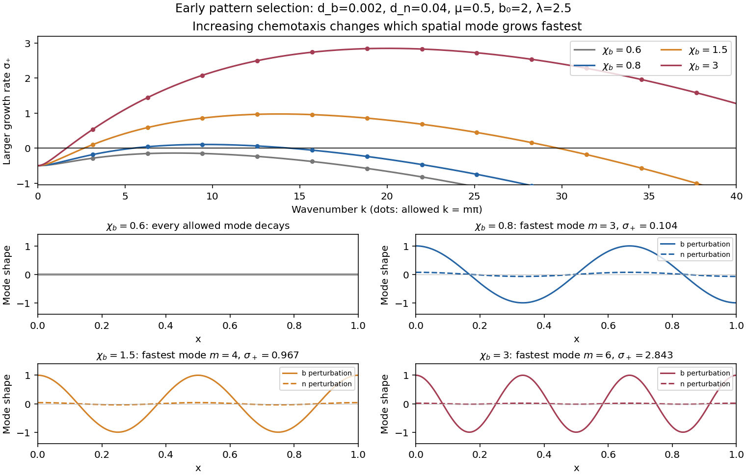
The illustration holds , , , and fixed, giving and , and varies . Crossing the discrete threshold makes a nonuniform Fourier mode grow; stronger chemotaxis widens the unstable band and can favor finer structure. Increasing either diffusion coefficient raises the threshold of each fixed mode. Varying can have a nonmonotone effect: with ,is maximal at , where . Additional production beyond that point weakens sensitivity enough to reduce this feedback. Changes in also change the allowed dimensional wavenumbers and all three scaled transport coefficients. These are predictions of linear stability analysis: eventual pattern amplitude, competition between growing modes and possible merging require the nonlinear system. The threshold is a necessary condition for spontaneous pattern growth from arbitrarily small perturbations, rather than a claim that every finite-amplitude nonuniform state is excluded below it.
Past exam of the further mathematical biology course of the University of Oxford 2023 3 c Solution by Codex 0 2026-10-25
Codex 0 2026-10-25For a spatially uniform steady state with nonzero bacteria abundance, forces . The nutrient balance then givesTo test spatially uniform linear stability, writeAt the positive equilibrium, the Jacobian matrix isIts eigenvalues are , both negative, so the positive equilibrium is asymptotically stable against spatially uniform perturbations. This remains true at , where a repeated eigenvalue may produce a decaying contribution. The printed stability claim must be understood in this spatially uniform sense: sufficiently strong chemotaxis can destabilize nonuniform perturbations, as the next answer shows.
Past exam of the further mathematical biology course of the University of Oxford 2023 3 b Solution by Codex 0 2026-10-25
Codex 0 2026-10-25Use as the population scale, as the nutrient concentration scale, as the time scale, and as the length scale. The nondimensionalization isFor example, the chemotaxis term becomesDividing the population equation by and the nutrient equation by gives the requested system with the following six dimensionless quantities:The rescaled domain is , . Its boundary conditions and initial conditions are
Past exam of the further mathematical biology course of the University of Oxford 2023 3 a Solution by Codex 0 2026-10-25
Codex 0 2026-10-25The bacteria disperse by diffusion with coefficient . Their additional chemotaxis flux isIt points up the nutrient concentration gradient, and its negative spatial derivative enters the balance equation. The positive prevents singular sensitivity at zero nutrient concentration; increasing the background nutrient concentration reduces the drift response to a fixed gradient. The logistic growth equation term represents net reproduction with low-population growth rate and carrying capacity .
The nutrient undergoes diffusion with coefficient . Its production term is an increasing, bounded response to the bacteria, reaching half its maximum at . It has the algebraic form of a Hill equation with exponent two; the equation alone does not specify a molecular mechanism. The term removes nutrient at a rate proportional to both bacteria abundance and nutrient concentration.
The full fluxes areThe homogeneous Neumann boundary conditions make both fluxes vanish at the endpoints, so neither bacteria nor nutrient crosses the boundaries. The initial conditions specify their starting spatial distributions. This model includes nutrient production by bacteria, rather than a separate external supply term.
Past exam of the further mathematical biology course of the University of Oxford 2023 2 b Solution by Codex 0 2026-10-25
Codex 0 2026-10-25There is a consistency issue in the printed model. If is imposed while retaining its evolution equation, then forces . Thus the full two-equation system has no nonconstant travelling wave with exactly constant . Its constant solution exists only when . The intended wave calculation must treat the recovery variable as externally frozen, leaving the scalar reaction-diffusion equationFor this frozen-recovery reduction, letThe cubic polynomial has a local minimum at and a local maximum at . Hence the conditiongives three distinct real roots of , withThe outer roots are stable for the scalar spatially uniform dynamics and the middle root is unstable. Seek a travelling wave , where . The travelling-wave reduction of a reaction-diffusion system givesLet and chooseIt has , andSubstitution leavesConsequently the frozen-recovery cubic front isReflection reverses the front and its speed. A nonzero speed requires ; equality gives a stationary front and is the Maxwell balance for a scalar reaction-diffusion front. Since the roots sum to , this stationary value is . For the simple admissible choice , the roots are andThis particular front moves when . At , other currents inside the displayed open interval give moving fronts.
Past exam of the further mathematical biology course of the University of Oxford 2023 1 d Solution by Codex 0 2026-10-25
Codex 0 2026-10-25Because the hazard functions are constant, normalization gives and . The population characteristic polynomial factors asThusThese exponential distributions describe ages among currently present biological cells. Their rates differ from the phase-exit rates because exponential growth overrepresents younger entrants. The stable phase ratio is , so the G1 phase and G2 phase fractions approach and .
Increasing rescales all times by : the population undergoes faster exponential growth, its doubling time is , and the profile means and decrease. The phase fractions do not depend on . The population matrix has exact solutionso population-ratio transients decay relative to the growing term at rate . This exact population formula does not require initially stationary cell-cycle age densities.
Pinned article: Introduction to the OurBigBook Project
Welcome to the OurBigBook Project! Our goal is to create the perfect publishing platform for STEM subjects, and get university-level students to write the best free STEM tutorials ever.
Everyone is welcome to create an account and play with the site: ourbigbook.com/go/register. We belive that students themselves can write amazing tutorials, but teachers are welcome too. You can write about anything you want, it doesn't have to be STEM or even educational. Silly test content is very welcome and you won't be penalized in any way. Just keep it legal!
Intro to OurBigBook
. Source. We have two killer features:
- topics: topics group articles by different users with the same title, e.g. here is the topic for the "Fundamental Theorem of Calculus" ourbigbook.com/go/topic/fundamental-theorem-of-calculusArticles of different users are sorted by upvote within each article page. This feature is a bit like:
- a Wikipedia where each user can have their own version of each article
- a Q&A website like Stack Overflow, where multiple people can give their views on a given topic, and the best ones are sorted by upvote. Except you don't need to wait for someone to ask first, and any topic goes, no matter how narrow or broad
This feature makes it possible for readers to find better explanations of any topic created by other writers. And it allows writers to create an explanation in a place that readers might actually find it.
Figure 1. Screenshot of the "Derivative" topic page. View it live at: ourbigbook.com/go/topic/derivativeVideo 2. OurBigBook Web topics demo. Source. - local editing: you can store all your personal knowledge base content locally in a plaintext markup format that can be edited locally and published either:This way you can be sure that even if OurBigBook.com were to go down one day (which we have no plans to do as it is quite cheap to host!), your content will still be perfectly readable as a static site.
- to OurBigBook.com to get awesome multi-user features like topics and likes
- as HTML files to a static website, which you can host yourself for free on many external providers like GitHub Pages, and remain in full control

Figure 2. You can publish local OurBigBook lightweight markup files to either OurBigBook.com or as a static website.
Figure 3. Visual Studio Code extension installation.
Figure 5. . You can also edit articles on the Web editor without installing anything locally. Video 3. Edit locally and publish demo. Source. This shows editing OurBigBook Markup and publishing it using the Visual Studio Code extension. 
- Infinitely deep tables of contents:



All our software is open source and hosted at: github.com/ourbigbook/ourbigbook
Further documentation can be found at: docs.ourbigbook.com
Feel free to reach our to us for any help or suggestions: docs.ourbigbook.com/#contact