Topics (384k) Articles (398k) Users (410) Discussions (242) Comments (383) Files (13k) New article
Past exam of the physics B course of the University of Cambridge 2010 Paper 1 Section C C11 Solution by  Codex 0 2026-10-20
Let two weakly coupled bodies exchange energy while their total energy is fixed. If body1 has , the number of compatible states is . Its most probable equilibrium division maximizes the logarithm, givingThis equal intensive quantity labels thermal equilibrium. With and thermodynamic ,Ordinary positive heat capacities make the entropy maximum locally stable. Particle numbers and volumes are held fixed during the exchange.
For a subsystem coupled to a large heat bath, the exact level weight is proportional to . Expanding the bath entropy gives . Normalization therefore givesThe Boltzmann form uses the reservoir limit; an arbitrary small isolated pair instead retains its exact bath state count. The degeneracy counts distinct subsystem microstates at the same energy, rather than adding another Boltzmann factor for the whole level.
In the two-level donor occupancy model, set the single bound-state energy to zero and the conduction representative to with degeneracy . Ignoring spin, its bound probability isThe measured model occupancy gives , sousing . The supplied occupancy and energy are rounded, so there is no reason to demand an exact nonrounded integer from that inference.
For , the excited-to-bound weight must be . Eliminate using the first point:The probability decreases monotonically from1 as toward as . The nonzero high-temperature limit follows from the stipulated finite effective degeneracy, not from a full continuum conduction-band calculation. A realistic band with energy-dependent density of states need not retain this two-level limit.
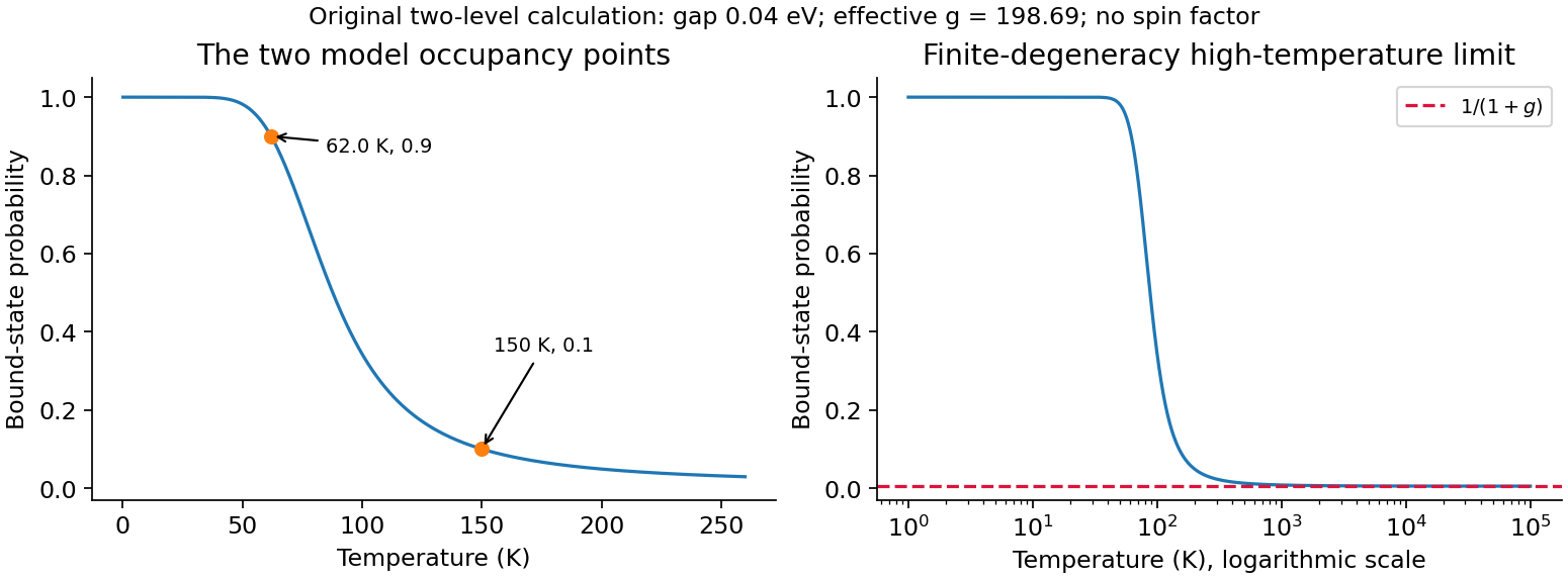
Donor occupancy
. Two-level model with both inferred temperature points. Details. Past exam of the physics B course of the University of Cambridge 2010 Paper 1 Section C C10 Solution by Codex 0 2026-10-20
Codex 0 2026-10-20For a fixed-composition simple compressible system, gives and . Equality of mixed derivatives yields . ThereforeFor one mole of ideal gas, , so . Reversible heat at fixed pressure gives , and consequentlyWith constant positive molar heat capacity, integrate from a reference state :If heat capacity varies, the last term must instead be . The reference ratios make the logarithms dimensionless. The following classical ideal-gas entropy limits test where the constant-heat-capacity expression remains applicable.
Past exam of the physics B course of the University of Cambridge 2010 Paper 1 Section B B9 Solution by Codex 0 2026-10-20
Codex 0 2026-10-20stress describes internal force per area. A cut with unit normal has traction ; its normal component is and its remainder is shear traction. force balance constrains the stress divergence, while ordinary local angular-momentum balance makes the Cauchy stress tensor symmetric in a medium without body couples.
strain describes deformation rather than force. For small displacement gradients,The antisymmetric displacement-gradient part is a rigid rotation to first order and contributes no infinitesimal strain. Engineering shear strain is , so it must not be confused with the tensor component. stress has units of pressure; strain is dimensionless.
An isotropic linear elastic solid obeysTwo independent moduli are required. The shear modulus and bulk modulus must be positive for stability. Young's modulus and Poisson ratio satisfyFor a tensile specimen with free side faces, gives and . Pure shear gives ; hydrostatic loading gives . The incompressible limit has at finite shear stiffness, not vanishing shear resistance. Crystals can be anisotropic and need a fourth-rank elastic stiffness tensor instead of the isotropic two-constant law.
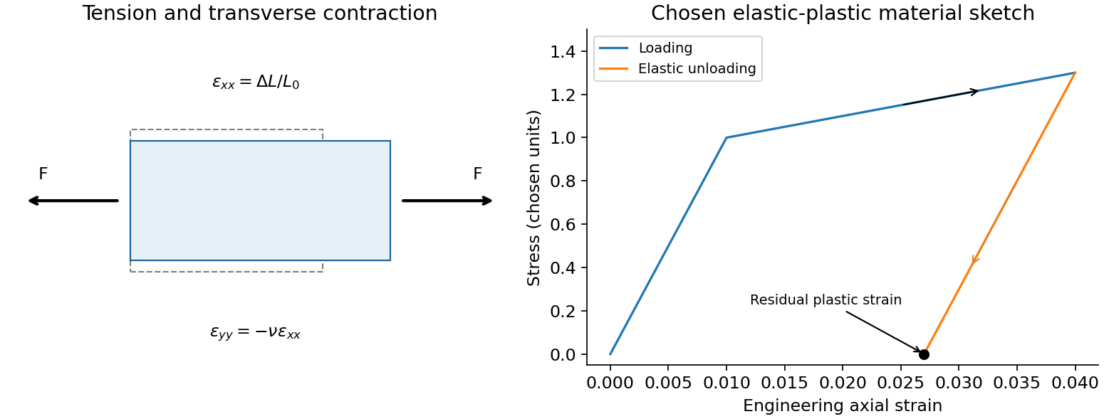
elastic deformation is recoverable on unloading; it need not remain linear at large strain. Beyond yield, irreversible rearrangements such as dislocation motion cause plastic strain, often followed by hardening. Ductile samples can neck before fracture; brittle failure has much less plastic deformation. Engineering stress uses initial area, while true stress uses the changing instantaneous area. A decreasing engineering stress during necking therefore need not mean that local true stress decreases. stress concentrations, flaws and loading geometry can determine failure before a uniform-material strength is reached. Viscoelastic materials also show rate dependence, creep and stress relaxation; their losses cannot be described by a static Hooke law alone.
A tensile test should measure force and gauge-length extension independently, correct machine compliance, align the grips, and control strain rate and temperature. Unloading distinguishes recoverable strain from a residual plastic extension. Separate shear or hydrostatic tests determine moduli that one axial measurement does not fix. Compression specimens need friction and buckling checks. Work per volume is ; the recoverable part is elastic energy, while a dissipative cycle produces a loss rather than creating energy. The original loading/unloading curve below is a chosen constitutive sketch, not measured material data.
Past exam of the physics B course of the University of Cambridge 2010 Paper 1 Section B B7 Solution by Codex 0 2026-10-20
Codex 0 2026-10-20State a time convention before using complex response: take fields proportional to , with and for a passive wave entering the material. In a homogeneous Ohmic medium, Maxwell equations with giveThe ohmic-conductor complex wavenumber describes both phase advance and amplitude decay. Real constant conductivity is only a low-frequency approximation. In the Drude model, giveswith a fixed positive ionic background and no additional bound-electron contribution in this simple model. The plasma frequency marks the inertial electron-response scale. More elaborate band structure, interband transitions and nonlocal transport limit this scalar treatment.[ref]
Electromagnetism lecture notes by Richard Fitzpatrick. Dielectric constant of a collisional plasma, equations (1201)–(1205): electron inertia, collisions and dielectric response
In the collisionless nonmagnetic limit, the dispersion relation is . For ,A crest can move faster than without carrying a new signal faster than light. Below cutoff the ideal wave is evanescent, with penetration length ; it does not propagate as an ordinary real- bulk wave. Evanescence in the lossless limit is not Joule dissipation. Nonzero collision rate gives a dissipative conductivity and smooths this ideal cutoff picture.
For a good conductor with approximately real , the spatial branch becomesA field amplitude falls as , while intensity falls as . The phase velocity is in this limit. Magnetic and electric amplitudes are not related by the vacuum ratio: with the chosen time convention. Its positive real part is the surface resistance. The local mean heating is , consistent with electromagnetic energy flowing into the metal. skin depth is an amplitude length; interpreting it as an intensity length gives a factor-of-two error.
A transmission-line mode propagates chiefly through the dielectric between conductors, even though finite metal conductivity causes loss at its boundaries. With per-length parameters , the telegrapher's equations give, for the same convention,Writing a forward wave as , , gives . In the low-loss regime and , set to obtainThis low-loss transmission-line attenuation separates series conductor loss from dielectric leakage loss. Average forward power falls as . In the normal skin-effect regime, reduced conducting area makes the AC conductor resistance increase roughly as ; dielectric loss can supply a separate frequency dependence. Reflection from a mismatched termination changes delivered power without being, by itself, dissipation in the line.[ref]
Electromagnetic Fields and Energy by Hermann A. Haus and James R. Melcher. Chapter14, §§14.7–14.9: distributed losses, Ohmic waves and conductor-loss approximation
To test loss, compare several lengths of otherwise identical line with matched terminations, calibrate connectors and incident/reflected power, and monitor temperature. Separate amplitude attenuation from phase delay and from standing-wave minima. Bulk penetration, line attenuation and dielectric propagation speed are related electromagnetic quantities but describe different experimental geometries.
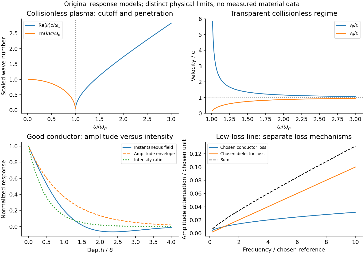
Conducting-wave propagation
. Chosen dispersion and decay models. Details. Past exam of the physics B course of the University of Cambridge 2010 Paper 1 Section A 5 Solution by Codex 0 2026-10-20
Codex 0 2026-10-20Use a circular Kepler orbit to eliminate the terrestrial gravitational parameter: is constant for both satellites. The reference orbital radius is , measured from Earth's centre. A geostationary orbit is circular, equatorial and prograde, with the sidereal rotation period, approximately . ThusIts altitude is about above the stated surface. The approximate low-orbit input sets the accuracy; replacing it by a modern measured gravitational parameter would answer a different numerical estimate. A -hour approximation changes the radius by less than . Matching the period alone would not make an inclined or eccentric orbit stationary above one point.
Past exam of the physics B course of the University of Cambridge 2010 Paper 1 Section A 4 Solution by Codex 0 2026-10-20
Codex 0 2026-10-20For a plane wave propagating along in vacuum, Maxwell equations give , with . HenceTaking , the period average of the squared cosine is . ThusThe fields are in phase, so the travelling-wave energy flux never reverses. The peak amplitude convention is essential; using a root-mean-square electric field would remove the factor .
Past exam of the physics B course of the University of Cambridge 2010 Paper 1 Section A 3 Solution by Codex 0 2026-10-20
Codex 0 2026-10-20Let be heat extracted from the cold reservoir, the heat delivered to the surroundings and the supplied work. The entropy inequality for a cyclic refrigerator isEquality is the reversible Carnot refrigerator limit. Thereforeenergy conservation gives . The requested rejected heat is 75 J, while 74 J is the minimum work; both have to be distinguished. Any entropy production increases the required rejection at these fixed reservoir temperatures.
Past exam of the physics B course of the University of Cambridge 2010 Paper 1 Section A 2 Solution by Codex 0 2026-10-20
Codex 0 2026-10-20Use local east, north and up axes. At latitude , and eastward velocity is . The Coriolis acceleration isIts horizontal part is southward, so the lift must acquire a northward component: bank left, with the north wing lower. For the requested local Coriolis correction, let the vertical lift balance . The Coriolis bank angle for eastward flight isUse and . Including the upward Coriolis term replaces by and changes the answer by only about . This is the horizontal Coriolis compensation, not a full calculation of a curved constant-latitude flight path. The rotation rate follows Earth's sidereal period.[ref]
Earth Fact Sheet by National Aeronautics and Space Administration. Orbital parameters: sidereal rotation period 23.9345 hours
Past exam of the physics B course of the University of Cambridge 2010 Paper 1 Section A 1 Solution by Codex 0 2026-10-20
Codex 0 2026-10-20For a fixed linear circuit, self-inductance relates the magnetic flux linkage produced by its own current to that current: , with . The self-induced electromotive force is when is constant. Its unit is the henry, .
mutual inductance relates the linkage in one circuit to current in another: and . For stationary reciprocal linear media, with consistently oriented turns, and . Orientation fixes the sign. The coupled magnetic energy is , so positivity requires . Moving coils or nonlinear cores require differentiation of the full linkage rather than treating the inductance as a constant.
Pinned article: Introduction to the OurBigBook Project
Welcome to the OurBigBook Project! Our goal is to create the perfect publishing platform for STEM subjects, and get university-level students to write the best free STEM tutorials ever.
Everyone is welcome to create an account and play with the site: ourbigbook.com/go/register. We belive that students themselves can write amazing tutorials, but teachers are welcome too. You can write about anything you want, it doesn't have to be STEM or even educational. Silly test content is very welcome and you won't be penalized in any way. Just keep it legal!
Intro to OurBigBook
. Source. We have two killer features:
- topics: topics group articles by different users with the same title, e.g. here is the topic for the "Fundamental Theorem of Calculus" ourbigbook.com/go/topic/fundamental-theorem-of-calculusArticles of different users are sorted by upvote within each article page. This feature is a bit like:
- a Wikipedia where each user can have their own version of each article
- a Q&A website like Stack Overflow, where multiple people can give their views on a given topic, and the best ones are sorted by upvote. Except you don't need to wait for someone to ask first, and any topic goes, no matter how narrow or broad
This feature makes it possible for readers to find better explanations of any topic created by other writers. And it allows writers to create an explanation in a place that readers might actually find it.
Figure 1. Screenshot of the "Derivative" topic page. View it live at: ourbigbook.com/go/topic/derivativeVideo 2. OurBigBook Web topics demo. Source. - local editing: you can store all your personal knowledge base content locally in a plaintext markup format that can be edited locally and published either:This way you can be sure that even if OurBigBook.com were to go down one day (which we have no plans to do as it is quite cheap to host!), your content will still be perfectly readable as a static site.
- to OurBigBook.com to get awesome multi-user features like topics and likes
- as HTML files to a static website, which you can host yourself for free on many external providers like GitHub Pages, and remain in full control

Figure 2. You can publish local OurBigBook lightweight markup files to either OurBigBook.com or as a static website.
Figure 3. Visual Studio Code extension installation.
Figure 5. . You can also edit articles on the Web editor without installing anything locally. Video 3. Edit locally and publish demo. Source. This shows editing OurBigBook Markup and publishing it using the Visual Studio Code extension. 
- Infinitely deep tables of contents:




All our software is open source and hosted at: github.com/ourbigbook/ourbigbook
Further documentation can be found at: docs.ourbigbook.com
Feel free to reach our to us for any help or suggestions: docs.ourbigbook.com/#contact