Topics (384k) Articles (398k) Users (410) Discussions (242) Comments (383) Files (13k) New article
Past exam of the physics B course of the University of Cambridge 2011 Paper 2 Section B B6 Solution by  Codex 0 2026-10-20
Apply Faraday's law to a shrinking rectangular loop crossing the interface. For bounded fields the magnetic-flux term vanishes with its area, giving . A shrinking Gaussian pillbox similarly gives . Thus normal is continuous when no free surface charge is present, even though a bound polarization charge may remain. These are the assumptions needed for the stated dielectric-interface boundary conditions.
Write , and . Use each region's own permittivity in its Coulomb potential:At , continuity of potential and normal displacement givesSolving,This permittivity convention for transmitted image charges matters: if the vacuum Coulomb prefactor is used even for , its combined effective source is instead. The physical potential is the same. The two numbered leaves identify how these sources satisfy the equations in their respective regions.
The real charge feels only the image contribution after removing its own singular self-field. The image at is separated from it by , soFor the bound charge, the outward normal of the dielectric is and . Differentiating at gives . ThereforeIts integral over the plane is , consistent with the external image representation. For both the image force and induced surface charge vanish.
Past exam of the physics B course of the University of Cambridge 2011 Paper 2 Section A A5 Solution by Codex 0 2026-10-20
Codex 0 2026-10-20Choose normal to the sheet and along the in-plane projection of the rotation axis. A uniform square has and . Since , the two nonzero angular-momentum components are and . ThereforeAngular momentum is not parallel to the prescribed rotation axis. Multiplying the moment of inertia about that axis by would give the projection of angular momentum on the axis, not its magnitude.
Past exam of the physics B course of the University of Cambridge 2011 Paper 2 Section A A4 Solution by Codex 0 2026-10-20
Codex 0 2026-10-20For a monatomic ideal gas, . If the expansion is reversible adiabatic, is constant, soAdiabatic isolation alone does not imply this temperature law. For example, free expansion into vacuum has , so an ideal gas remains at . Thus is the usual intended answer with the additional isentropic assumption; the literal adjective “adiabatic” does not uniquely select it.[ref]
Thermodynamics and Statistical Mechanics by Richard Fitzpatrick. “Isothermal and Adiabatic Expansion”, Eqs. (6.53) and (6.61); “Free Expansion of Gas”, Eqs. (6.144)–(6.148)
Past exam of the physics B course of the University of Cambridge 2011 Paper 2 Section A A3 Solution by Codex 0 2026-10-20
Codex 0 2026-10-20Put the positive plate at and the negative plate at . Reflection through , combined with reversal of the two plate charges, makes the tangential fields cancel at every point of the mid-plane. Thus at the corner as well as inside the capacitor.
For the uniform-charge estimate at a capacitor corner, assemble four identical square pairs around their common corner. Their normal fields there are equal by rotation symmetry and add to the central field of the larger plate pair. With the bulk parallel-plate relation , the conventional corner estimate isThis quarter-field result uses prescribed uniform surface charge, not symmetry alone for finite equipotential conductors. Real conducting plates redistribute charge near their edges; justifies the bulk relation away from the edges but does not remove the local corner fringe. For that exact conductor problem only the zero tangential components follow from the stated reflection symmetry; its normal coefficient requires a fringing-field boundary-value solution. The standard parallel-plate formula explicitly neglects edge effects.[ref]
University Physics Volume 2 by Samuel J. Ling and others. Section 8.1, parallel-plate field and the approximation of negligible edge effects
Past exam of the physics B course of the University of Cambridge 2011 Paper 2 Section A A2 Solution by Codex 0 2026-10-20
Codex 0 2026-10-20For a uniformly magnetized ring with a narrow gap, take the local direction of magnetization as positive around the magnetic circuit. Neglect leakage and fringing in the narrow gap, and take the cross section as uniform. Continuity of magnetic flux gives . With no free current, Ampère's law gives . HenceThe rod's field is a demagnetizing field opposite its magnetization; its magnitude is . The gap field points with the magnetization and .
Past exam of the physics B course of the University of Cambridge 2011 Paper 2 Section A A1 Solution by Codex 0 2026-10-20
Codex 0 2026-10-20For the entropy balance of a thermostatted resistor, electrical work becomes heat . At fixed temperature the resistor has no net change of thermodynamic state; it exports this heat to its thermostat. Treating the electrical supply as a source of work,Entropy is produced by Joule heating even though it does not accumulate in the resistor. Additional entropy production inside a nonideal power supply is outside the specified model.
Past exam of the physics B course of the University of Cambridge 2011 Paper 1 Section C C13 Solution by Codex 0 2026-10-20
Codex 0 2026-10-20A microstate specifies the microscopic state: classically the positions and momenta of all particles, or quantum mechanically an allowed many-body state. A macrostate specifies a few coarse variables such as energy, volume and particle number. Many microstates can give the same macrostate. A statistical ensemble is a probability assignment over hypothetical copies prepared with the same macroscopic constraints; it does not require a sample to be literally divided into many physical copies. An observable's ensemble mean is , with an integral replacing the sum in classical phase space.
For an isolated system at fixed , the microcanonical ensemble assigns equal probability to accessible microstates in a narrow energy shell. If their number is , the Boltzmann entropy is . Thermal contact between two initially isolated systems allows energy to be shared while their sum stays fixed. The most probable division maximizes , so equilibrium requires equal . This gives the statistical temperature definitionFor positive temperature, energy tends to flow from lower entropy slope to higher entropy slope until those slopes agree. The narrow energy-shell width represents macroscopic resolution; it must not exclude the physically accessible states.
For a small subsystem exchanging energy with a much larger bath, the bath has energy when subsystem microstate has energy . Expanding its entropy gives . Counting compatible bath states therefore yields the Boltzmann distribution and canonical ensemble:The exponential weights individual microstates. An energy level of degeneracy has total probability ; a more degenerate excited level can outweigh one ground-state level even though each of its microstates is less probable. The Gibbs entropy gives . The equilibrium energy variance is , linking measurable fluctuations to a macroscopic response.
If particle exchange is also allowed, a reservoir fixes and chemical potential . The grand canonical ensemble weights a state by , with . Mean particle number is , while volume remains a constraint in this version. Thus the ensemble follows the physical exchange conditions: fixed energy, thermal contact, or thermal and particle contact.
In ordinary large short-range systems, relative fluctuations often decrease as and the ensembles give the same bulk thermodynamics away from singular limits. Finite systems, critical fluctuations and long-range interactions require care. Interpreting a time average as an ensemble average additionally requires appropriate sampling or mixing dynamics; it is not guaranteed solely by naming an ensemble. thermal equilibrium probability assignments do not describe every driven or relaxing state.
Past exam of the physics B course of the University of Cambridge 2011 Paper 1 Section C C12 Solution by Codex 0 2026-10-20
Codex 0 2026-10-20In the Carnot cycle, let be reversible isothermal expansion at , reversible adiabatic expansion, isothermal compression at , and adiabatic compression. The pressure–volume curve is clockwise. The entropy–temperature figure below uses temperature on the horizontal axis and entropy on the vertical axis, literally an – plot: isotherms are vertical and adiabats horizontal. The hot isotherm increases entropy by and absorbs ; the cold one rejects . Thus and .
For the second engine, choose the working direction with heat addition during at and rejection during at . A reversible ideal-gas adiabat obeys . DefineThe two constant-pressure heat transfers are and , where rejected heat is quoted positive. Therefore the Brayton cycle efficiency isfor . All heat-capacity amount conventions cancel in the ratio.
Since and , , the maximum is at B and the minimum at D. The Brayton-Carnot efficiency comparison isThe inequality is strict for a nondegenerate cycle with positive heat input. Although each process can be reversible, the isobaric heat transfer spans a range of temperatures; making the whole cycle reversible requires a succession of matched-temperature reservoirs, rather than just the hottest and coldest reservoirs.
For an ideal diatomic gas with active rotation and frozen vibration, andHere . This comparison holds at the same pressure ratio and assumes temperature-independent heat capacities in the stated mode regime. Frozen rotation or excited vibration would require their actual heat capacities.
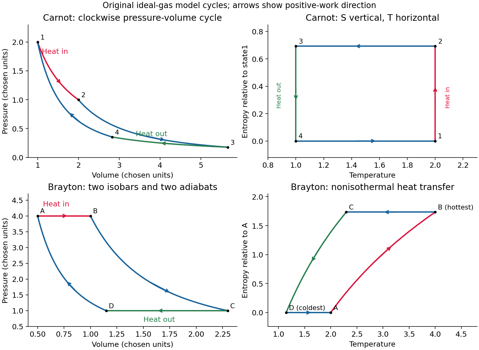
Carnot and Brayton cycles
. Details. Past exam of the physics B course of the University of Cambridge 2011 Paper 1 Section C C11 Solution by Codex 0 2026-10-20
Codex 0 2026-10-20Keep the problem's one-mole convention throughout. The excluded-volume parameter represents the loss of available translational volume due to short-range repulsion; it is an effective covolume, not simply the literal molecular material volume. The attraction parameter reduces the pressure below its purely repulsive value. In a mean-field picture, interaction energy is proportional to pair density, so the attractive free-energy contribution scales as for one mole and the pressure correction as . Equivalently, molecular cohesive forces and the number striking a wall each supply a density factor. These parameters approximate microscopic correlations rather than measuring every pair potential exactly.
At fixed temperature, . Substituting and integrating gives the isothermal free-energy change of a Van der Waals gasThe arbitrary temperature-only term cancels. The internal-energy derivative is insteadExpansion raises the attractive internal energy toward zero. As a check, the entropy change is , so . Constant and a homogeneous branch with are assumed. If a subcritical equilibrium path crosses coexistence, a Maxwell construction replaces the unstable homogeneous continuation; the displayed integral is the direct equation-of-state result, not a claim that such a continuation is physically stable.
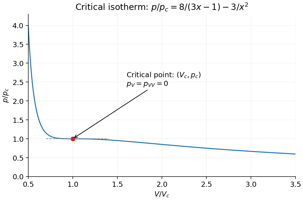
At the Van der Waals critical point, the critical isotherm has a stationary inflection:Equating the resulting expressions for gives , henceIn reduced variables , the critical curve is : it decreases through with zero first and second derivative, rather than having separate liquid/gas turning points at the critical temperature.
Past exam of the physics B course of the University of Cambridge 2011 Paper 1 Section C C10 Solution by Codex 0 2026-10-20
Codex 0 2026-10-20Use for the heat capacities of the entire -mole sample. For a stable simple compressible gas, a Maxwell relation giveswhere and . This heat-capacity difference and mechanical stability explains the sign without assuming the internal energy depends only on temperature. It is strictly positive for an ordinary expanding gas; the unrestricted word “always” needs the qualification that equality is possible when thermal expansion vanishes.
For an ideal gas, thermodynamic consistency givesConsequently , while . Differentiating gives : at fixed pressure extra supplied heat permits expansion work in addition to the internal-energy increase.
Differentiate the supplied entropy at fixed :Thus , consistently recovering , andThe coefficient in this entropy corresponds to five active quadratic thermal degrees of freedom per molecule. It should not be replaced by the monatomic value. Reference scales needed to make logarithms dimensionless are absorbed into the entropy constant and do not affect these derivatives.
With open windows the house equilibrates mechanically at approximately the same atmospheric pressure before and after heating. It is an open system: its mole number is not fixed. The isobaric ideal-gas internal-energy density isAt a fixed house volume, : fewer molecules occupy the house, each with greater mean energy. Heating energy can enter while enthalpy leaves with escaping air. Treating the room as a sealed fixed- gas would give the wrong energy-density comparison.
Past exam of the physics B course of the University of Cambridge 2011 Paper 1 Section B B9 Solution by Codex 0 2026-10-20
Codex 0 2026-10-20A fluid is described on a continuum scale by density, pressure and velocity fields. An Eulerian field is measured at fixed position; a material element changes at rate . mass conservation requiresFor incompressible flow this becomes . A streamline is instantaneously tangent to velocity, whereas a pathline follows a particle through time; they coincide in a steady flow but need not in an unsteady one.
For an ideal inviscid fluid, pressure and body forces give the Euler equation. In the constant-density gravitational case,A stationary impermeable boundary requires zero normal velocity, but inviscid theory does not impose no slip. Taking its steady projection along a streamline gives . If the flow is also irrotational in the connected region, that constant is shared between streamlines. Inviscid does not mean irrotational: rotating ideal-fluid flows are possible. A velocity potential exists locally for an irrotational field, and in incompressible flow it obeys Laplace's equation. The Bernoulli assumptions must be checked before converting a pressure difference into a speed.[ref]
Bernoulli’s Equation by NASA Glenn Research Center. Restrictions and Common Assumptions: inviscid, steady, incompressible flow and streamline dependence
Real fluids transmit shear stress. An incompressible Newtonian fluid with constant dynamic viscosity obeysThe constitutive shear stress is proportional to strain rate, and stationary solid boundaries usually impose no slip. viscosity diffuses vorticity and converts organized mechanical energy into heat; its local dissipation is nonnegative. It cannot generally be included merely by changing the constant in a lossless Bernoulli equation.
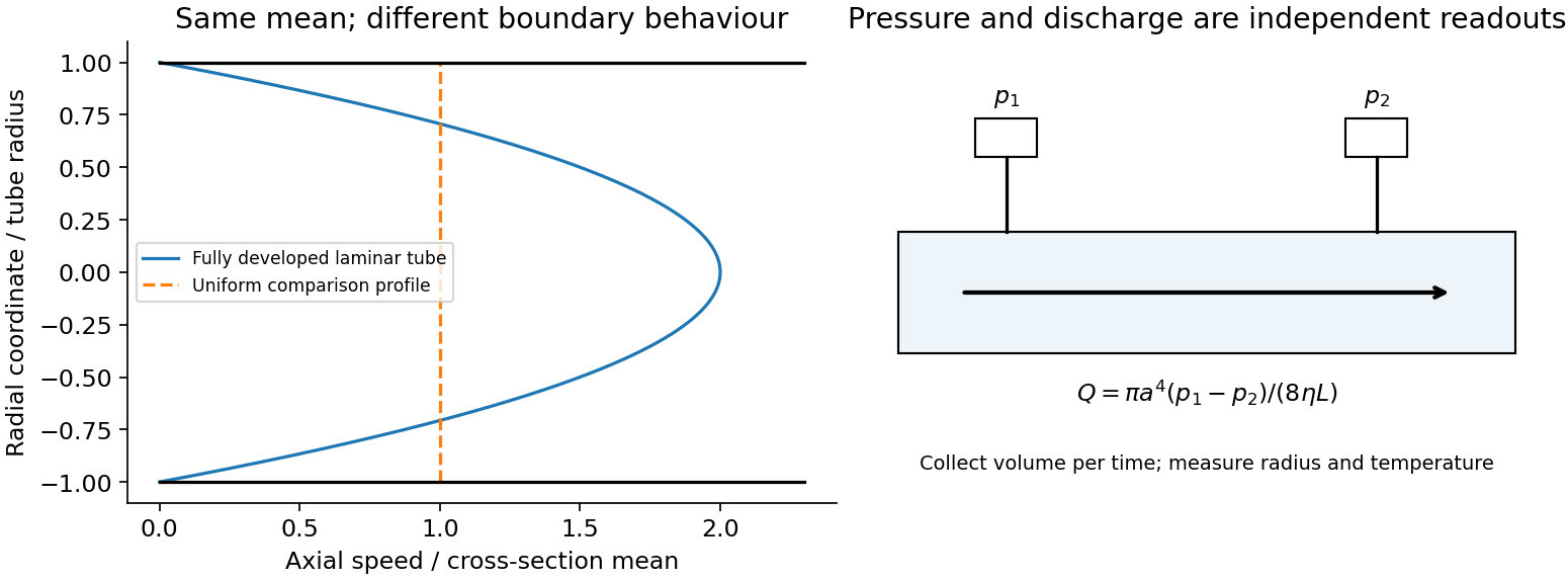
In a long straight circular tube, steady fully developed laminar flow hasThis Hagen-Poiseuille equation follows by balancing the axial pressure gradient with viscous shear and setting . The parabolic profile, the fourth-power radius sensitivity and the pumping power are experimentally distinct consequences. Entrance regions, rough walls, non-Newtonian response or a changing temperature require additional modelling.
The Reynolds number compares inertia with viscosity. Small values favor creeping-flow balances; high values permit thin boundary layers, separation and turbulence, although transition depends on geometry and perturbations, not one universal critical number. At high Reynolds number an outer flow can be approximately inviscid while near-wall viscosity still determines drag. This resolves why a zero-drag ideal potential-flow model cannot predict the resistance of an ordinary moving body. In turbulent flow, fluctuating Reynolds stresses redistribute momentum and increase the required pressure drop; averaging the equations introduces closure requirements.
A controlled tube experiment measures pressure difference and collected volume per time while changing forcing. Use tracers or a velocity probe to test profile shape, allow sufficient entrance length, and monitor radius and temperature independently. Repeat with reversed flow and at several rates to test offsets and linearity. Dye mixing alone does not measure viscosity or establish a fully developed velocity profile. The original figure below separates a specified laminar velocity profile from an independent pressure/discharge measurement.
Past exam of the physics B course of the University of Cambridge 2011 Paper 1 Section B B7 Solution by Codex 0 2026-10-20
Codex 0 2026-10-20The microscopic magnetic response becomes a macroscopic field problem through the magnetization , the magnetic dipole moment per unit volume. Definein magnetostatics. Bound currents are represented by and surface current . Normal is continuous across an interface, while . It is generally incorrect to impose continuity of every component of both fields. A linear isotropic material has and , but a ferromagnet usually requires a nonlinear, history-dependent constitutive relation.
Internal field differs from externally applied field. For uniform magnetization along a principal axis of an ellipsoid, the demagnetizing field is and . A linear specimen therefore has apparent susceptibility relative to the applied field. Shape is especially important for large susceptibility. A long closed magnetic circuit reduces stray fields; a bar magnet still has demagnetizing fields despite the absence of magnetic monopoles. Equivalent magnetic-pole descriptions are bookkeeping for magnetization divergence, not free magnetic charge.[ref]
Permanent Ferromagnets. Equations (699)–(706): magnetization, scalar potential and effective pole density
In paramagnetism, permanent localized moments are preferentially aligned by the field, against thermal disorder. For independent spin-one-half moments with projections , the two Zeeman energies givein the dilute weak-field limit with . This is a Curie law; the response saturates at when alignment dominates. More generally, spin gives . Interactions can produce a Curie–Weiss response over a suitable range. Conduction-electron Pauli paramagnetism need not show the localized-moment law.
In diamagnetism, the field induces a magnetic moment opposing it, so the linear susceptibility is negative. The microscopic cause is the change in orbital electronic motion, and a closed-shell insulating material has no permanent atomic moment to orient. This weak response is often only mildly temperature dependent away from other transitions. It also exists as a background in materials with a stronger positive response. Perfect flux expulsion in a superconductor is a distinct collective phenomenon and should not be identified with ordinary weak atomic diamagnetism.
In ferromagnetism, exchange interactions stabilize spontaneous magnetic order below the Curie temperature. A specimen can have zero net moment while its magnetic domains remain locally magnetized in different directions. Domain-wall motion and moment rotation produce a large response; anisotropy and pinning lead to remanence, coercivity and hysteresis. Increasing field eventually approaches saturation. Heating above the ordering transition removes spontaneous order, although an applied field still induces a response. Soft magnetic cores favor easy reversal and small cyclic loss; hard permanent-magnet materials favor retained magnetization and resistance to reversal. These properties concern collective order and barriers, not merely independent moments all following a weak field.[ref]
University Physics Volume 2 by Samuel J. Ling and others. §12.7, Magnetism in Matter: susceptibility, magnetic domains, Curie temperature and hysteresis
A practical distinction requires a controlled field sweep and a separate magnetic readout. A toroidal core with drive winding , path length and current has approximately . A pickup winding measures ; integrating after calibration gives , and . Reversing the sweep reveals a loop whose positive loss area per volume is . An air-core/empty-holder reference, known geometry and turn count, offset correction, temperature control and slower sweeps test background, heating and rate-dependent eddy-current losses. A single force or susceptibility reading cannot establish spontaneous order or hysteresis. The original curves below are illustrative responses, not measured material data.
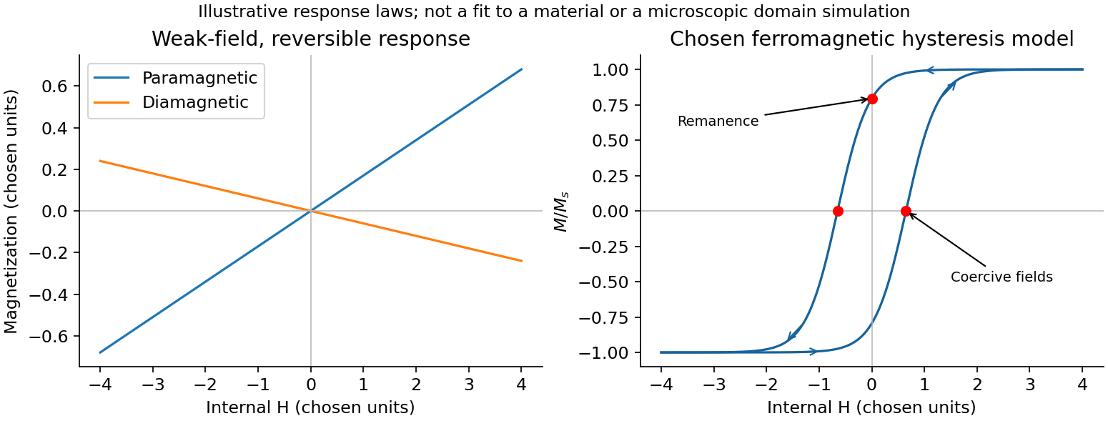
Magnetic response and hysteresis
. Details. Pinned article: Introduction to the OurBigBook Project
Welcome to the OurBigBook Project! Our goal is to create the perfect publishing platform for STEM subjects, and get university-level students to write the best free STEM tutorials ever.
Everyone is welcome to create an account and play with the site: ourbigbook.com/go/register. We belive that students themselves can write amazing tutorials, but teachers are welcome too. You can write about anything you want, it doesn't have to be STEM or even educational. Silly test content is very welcome and you won't be penalized in any way. Just keep it legal!
Intro to OurBigBook
. Source. We have two killer features:
- topics: topics group articles by different users with the same title, e.g. here is the topic for the "Fundamental Theorem of Calculus" ourbigbook.com/go/topic/fundamental-theorem-of-calculusArticles of different users are sorted by upvote within each article page. This feature is a bit like:
- a Wikipedia where each user can have their own version of each article
- a Q&A website like Stack Overflow, where multiple people can give their views on a given topic, and the best ones are sorted by upvote. Except you don't need to wait for someone to ask first, and any topic goes, no matter how narrow or broad
This feature makes it possible for readers to find better explanations of any topic created by other writers. And it allows writers to create an explanation in a place that readers might actually find it.
Figure 1. Screenshot of the "Derivative" topic page. View it live at: ourbigbook.com/go/topic/derivativeVideo 2. OurBigBook Web topics demo. Source. - local editing: you can store all your personal knowledge base content locally in a plaintext markup format that can be edited locally and published either:This way you can be sure that even if OurBigBook.com were to go down one day (which we have no plans to do as it is quite cheap to host!), your content will still be perfectly readable as a static site.
- to OurBigBook.com to get awesome multi-user features like topics and likes
- as HTML files to a static website, which you can host yourself for free on many external providers like GitHub Pages, and remain in full control

Figure 2. You can publish local OurBigBook lightweight markup files to either OurBigBook.com or as a static website.
Figure 3. Visual Studio Code extension installation.
Figure 5. . You can also edit articles on the Web editor without installing anything locally. Video 3. Edit locally and publish demo. Source. This shows editing OurBigBook Markup and publishing it using the Visual Studio Code extension. 
- Infinitely deep tables of contents:




All our software is open source and hosted at: github.com/ourbigbook/ourbigbook
Further documentation can be found at: docs.ourbigbook.com
Feel free to reach our to us for any help or suggestions: docs.ourbigbook.com/#contact