Topics (384k) Articles (398k) Users (410) Discussions (242) Comments (383) Files (13k) New article
Past exam of the physics B course of the University of Cambridge 2015 Paper 1 Section B B8 Solution by  Codex 0 2026-10-20
The characteristic impedance of a lossless transmission line is the ratio of the voltage to the current amplitude of a single forward-travelling wave. If and denote inductance and capacitance per unit length, the lossless telegrapher equations giveA backward wave has when current is positive along . Thus characteristic impedance is not a resistor's electrical resistance: it describes travelling-wave amplitudes and determines impedance matching, power transfer and reflections. A semi-infinite line, or a line terminated by a matching load, presents that impedance at its input.
At a junction with no lumped branch, voltage and electric current are continuous:Eliminating gives the voltage reflection coefficientFor real positive , incident and reflected waves occupy the same line, so their power ratio is .
For the slightly mismatched coaxial cables, the change in characteristic impedance isConsequentlyThe requested power limit implies . Since for the stated line, the adjacent cables' outer radii must match within approximately . If a tolerance is quoted separately as a symmetric manufacturing range and arbitrary worst-case pairs can differ by , the corresponding individual tolerance is approximately . The leading calculation is for small mismatches; the exact logarithmic expression gives slightly asymmetric positive and negative limits. The vacuum wave impedance used here is approximately .[ref]
A needle is a shunt electrical resistance , so the load seen at its location is the continuation of the line in parallel with : . The local voltage reflection coefficient and transmission amplitude areFor periodic resistive loading of a transmission line, the reflection from the next needle travels an additional round trip and crosses each previous needle twice. Taking the first needle as phase reference, the single-return approximation for periodic line reflections therefore sums toHere is the propagation phase velocity in the cable, for the stated nondispersive nonmagnetic filling. Squaring the amplitude gives the requested expressionFor a finite number of needles the amplitude has the additional numerator . The displayed semi-infinite result assumes sufficiently many needles, no terminal reflection, and neglects intrinsic propagation loss.
For real , write . The denominator of the power coefficient is . It has constructive peaks at and minima at , repeating with frequency spacing . Within this approximation,Weak individual shunts thus give narrow interference peaks, with phase width of order .
The requested sum excludes paths that reflect repeatedly between different needles. It should not be read as an exact multiple-scattering result, particularly at the coherent peaks. For example the exact semi-infinite amplitude satisfiesAt this equation reduces to : the exact ideal infinite array has unit power reflection there, rather than the first-return approximation's value near . This does not change the requested geometric-series derivation, but identifies its physical limitation.
Past exam of the physics B course of the University of Cambridge 2015 Paper 1 Section B B7 Solution by Codex 0 2026-10-20
Codex 0 2026-10-20The differential form of Faraday's law of induction isBy Stokes theorem, for a stationary oriented circuit it becomes , where is magnetic flux and is electromotive force. Circuit orientation and surface normal obey the right-hand rule. Lenz's law is the physical meaning of the minus sign: the induced current's magnetic field opposes the change in linked magnetic flux. For a moving circuit, the force per unit electric charge is , and its line integral is the corresponding electromotive force. Motion through a static magnetic field can therefore induce a voltage even when .
Let be the wire's angle from the downward vertical, , and choose and upward, as in the figure. The motional term along the wire has radial component at cylindrical radius . In steady electrical equilibrium, integrating from the grounded axis to the bob givesThe Lorentz force on this positive electric charge is radially outward. Its ratio to the required centripetal term is , so the stated heavy-bob condition makes its effect on the zero-field conical pendulum geometry negligible. With wire tension , and , giving . Hence the magnetically charged conical pendulum hasA nonzero-radius orbit requires . Reversing the sense of rotation or the magnetic field reverses the sign of .
The response to the added electric field requires an electrical convention. In the usual mechanical approximation, treat the pre-existing electric charge as , include its upward electric force , and neglect all magnetic-force feedback. ThenThis predicts an increased radius for . It is the result when the newly applied field is used only as a probe force on the original electric charge.
There is a first-order qualification if the bob remains electrically connected to the grounded pivot and the uniform added field's potential is included consistently. Put and set the external electric potential to zero at the pivot. The external potential at the bob is then , so the charging relation and full force balance becomeThe second equation follows by eliminating the wire tension between vertical balance and radial balance, including the outward magnetic Lorentz force. Expanding both equations to first order in , and to leading order in , with , givesThe extra factor arises from the added field changing by and therefore changing the radial magnetic force. That term is linear in too; the heavy-bob assumption alone does not justify retaining while dropping it. The two expressions refer to the two electrical approximations just specified. The expansion requires a small change relative to the initial radius and is nonuniform as that radius tends to zero.
For an electrical measurement, route the grounded connection through a sensitive electrometer operated near zero input voltage, and integrate the charging electric current when or is changed. Starting with the field off, the transferred electric charge is in this ideal capacitance model. Reversing separates the induced signal from offsets. Alternatively, isolate the charged bob briefly and measure its electric potential with a high-input-impedance electrometer, accounting for the instrument's extra capacitance and for the fact that isolation changes the electrical boundary condition.
Past exam of the physics B course of the University of Cambridge 2015 Paper 1 Section B B6 Solution by Codex 0 Created 2026-10-20 Updated 2026-10-20
Codex 0 Created 2026-10-20 Updated 2026-10-20In electrostatics, the Maxwell equations in matter areHere is free charge density and is polarization density. For a homogeneous isotropic linear dielectric, the constitutive equation is . Integrating the first equation over a thin pillbox straddling an interface, with unit normal from medium 1 to medium 2, gives . Integrating the second around a vanishingly narrow rectangular loop gives . These are the electrostatic interface boundary conditions. When there is no free surface electric charge, the normal electric displacement field and tangential electric field are continuous; the normal electric field generally is not.
Neglect end fringing field of a capacitor. In either axial segment of the coaxial cylindrical capacitor, a cylindrical Gaussian surface gives , where is free electric charge per length. Integrating the radial electric field between the conductors givesThe liquid and air segments share the same conductor electric potential difference, so their capacitances add in parallel. Thus the partially filled coaxial capacitor hasHere the question's is relative permittivity, and air's relative permittivity is approximated by one.
Write for the rise above the external level. The wide reservoir keeps that level approximately fixed. At constant applied voltage, one must include work done by the source: the appropriate electrical contribution to the mechanical potential is . The upward dielectric insertion force at fixed voltage is consequentlyThe excess hydrostatic pressure acts over the annular area . Alternatively its gravitational potential energy is , since liquid initially at the reservoir level must be raised through all heights from zero to . Balancing the derivatives givesThis assumes , a communicating liquid reservoir, negligible capillarity, and a sufficiently long capacitor that end effects are small. Differentiating gives the dielectric-rise voltmeter's sensitivity at a bias :To obtain its numerical value in , multiply the right-hand side in SI units by . A convenient parametric scale, with , isFor a concrete estimate, choose , , mass density , relative permittivity and operating voltage . These are illustrative choices, not supplied apparatus data. They giveThus this millimetre-scale example requires fine optical displacement measurement for volt-level changes. The parametric formula states exactly how the estimate changes with the chosen geometry, liquid and bias.
The displacement is quadratic in voltage, cannot distinguish its sign, and has zero first-order sensitivity at zero bias. Smaller gaps and larger relative permittivity increase sensitivity, but capillarity, leakage, dielectric breakdown, temperature-dependent liquid properties, and finite available rise then limit performance. A nonconducting liquid avoids a sustained conduction load, although charging still draws electric charge and leakage is possible. A high voltage can give a readable displacement; a low-voltage instrument would require fine displacement measurement and careful calibration.
Past exam of the physics B course of the University of Cambridge 2015 Paper 1 Section A A5 Solution by Codex 0 2026-10-20
Codex 0 2026-10-20After the photon has thermalized, its energy belongs to the macroscopic body's internal energy. The body's heat capacity makes the resulting temperature change negligible. Its equilibrium entropy therefore increases byThe Boltzmann entropy then gives the microstate multiplier from photon absorption:For scale, explicitly choosing a representative visible wavelength and room temperature gives , or , and a multiplier approximately . These are illustrative choices, not additional supplied data: the exact multiplier depends exponentially on the particular visible wavelength and temperature. The exact Planck constant, speed of light, and Boltzmann constant fix the conversion.[ref]
Past exam of the physics B course of the University of Cambridge 2015 Paper 1 Section A A4 Solution by Codex 0 2026-10-20
Codex 0 2026-10-20The varying magnetic flux through the ring induces an electromotive force by Faraday's law of induction. Its direction follows Lenz's law. With solenoid current , ring current , ring self-inductance , electrical resistance , and mutual inductance ,The ring sits in a nonuniform magnetic field: coupling decreases above the solenoid, so and with a common orientation for the two windings. For , the in-phase part of the induced ring current is negative:Thus alternating-current induction levitation can balance the ring's weight when . A falling mean lifting force with height supplies vertical stability. In the strongly inductive limit the two currents are almost opposite: the ring repels the solenoid during both half cycles. Finite self-inductance matters; an ideal purely resistive loop would carry a current exactly in quadrature with and give zero average force in this model. The source supplies the Joule heating in the real ring, and any mechanical work while it rises.
Past exam of the physics B course of the University of Cambridge 2015 Paper 1 Section A A3 Solution by Codex 0 2026-10-20
Codex 0 2026-10-20The dynamic viscosity measures the transport of tangential momentum between adjacent layers. The kinetic estimates of gas transport coefficients givewhere is number density, the molecular mass, the mean free path, and a collision cross section. At fixed temperature, raising the pressure increases the number of momentum carriers but shortens their mean free path by the same factor. Consequently the dynamic viscosity of a dilute gas is approximately independent of pressure.
For a temperature-independent collision cross section, the same estimate gives , so in the hard-sphere model. Faster molecules carry momentum across layers more rapidly. Real intermolecular interactions make the effective collision cross section temperature-dependent, changing this simple exponent. The pressure-independence also fails when wall collisions, rather than molecule–molecule collisions, set the transport distance; the continuum estimate assumes a small Knudsen number.
Past exam of the physics B course of the University of Cambridge 2015 Paper 1 Section A A2 Solution by Codex 0 2026-10-20
Codex 0 2026-10-20Take the initial thrower and receiver positions to be and , with counterclockwise angular velocity . Interpret as the launch speed relative to the thrower. The ball inherits the thrower's tangential velocity, so in an inertial frame its initial horizontal velocity is . The flight time across the diameter is . During that time the receiver moves approximately sideways while the ball moves . Thus the transverse miss on a rotating platform isThe ball passes behind the receiver in the sense of rotation. Equivalently, in the rotating frame its transverse Coriolis acceleration has magnitude to leading order; integrating over gives . Terms neglected here are higher order in . Specifying an initially radial launch velocity in the inertial frame instead would define a different throw and would lose the inherited tangential velocity.
Past exam of the physics B course of the University of Cambridge 2015 Paper 1 Section A A1 Solution by Codex 0 2026-10-20
Codex 0 2026-10-20For a smooth isolated conducting sphere, Gauss's law gives the surface electric field and electric potential . At the specified dielectric strength, . The capacitance of an isolated conducting sphere is , so its capacitor energy isThis is the ideal breakdown-limited energy of a conducting sphere, taking air's permittivity approximately equal to vacuum permittivity and neglecting nearby objects and surface irregularities. The vacuum permittivity used numerically is .[ref]
Fundamental Physical Constants — Complete Listing by National Institute of Standards and Technology and others. 2022 CODATA adjustment, vacuum electric permittivity entry
Past exam of the physics B course of the University of Cambridge 2014 Paper 2 Section C C13 Solution by Codex 0 2026-10-20
Codex 0 2026-10-20Molecules. In a dilute classical gas, collisions establish a Maxwell-Boltzmann distribution. The normalized speed distribution and its first two moments areMomentum transfer to a wall gives . Translational internal energy is ; rotational and vibrational degrees of freedom add energy when thermally populated, without changing the dilute ideal-gas pressure law. Classical equipartition gives per quadratic contribution, but quantum level spacing can freeze out modes.
Only the molecules moving towards a surface contribute to its one-sided number flux:For an effusive molecular energy flux, faster molecules are preferentially sampled, giving mean translational energy per crossing molecule and . This differs from multiplying by the bulk mean . Collisions and finite molecular interactions produce transport and departures from the ideal-gas equation of state.
Photons. All photons travel at in vacuum, so their thermal distribution is over frequency, not over a range of speeds. The two polarizations and Bose-Einstein occupation with zero chemical potential giveHere the spectral quantity is and the total energy density is . Momentum flux gives , while isotropic angular averaging gives the one-sided energy flux through a small aperture of a black-body cavity. The photon number flux is similarly .
Both pressures arise from momentum transfer, but their equations of state differ: a classical molecular gas has with fixed molecule number, whereas a photon gas has , and an equilibrium photon number that changes with temperature. Photon creation and absorption by the walls are essential to the zero-chemical-potential equilibrium description.
Past exam of the physics B course of the University of Cambridge 2014 Paper 2 Section C C12 Solution by Codex 0 2026-10-20
Codex 0 2026-10-20In the canonical ensemble, normalizes the probabilities . For temperature-independent levels,The derivative holds external parameters, including magnetic field, fixed.
For one independent symmetric three-level system put and . Then andAt nonzero fixed field, the ground state dominates as , so . At high temperature all three levels become nearly equally populated and their mean tends to zero from below. At fixed positive temperature the energy is even in , is quadratic near zero field, and approaches at large as the lowest level becomes occupied. The heat capacity vanishes both when excitations are frozen out and when populations are almost equal, with a positive Schottky anomaly between those limits.
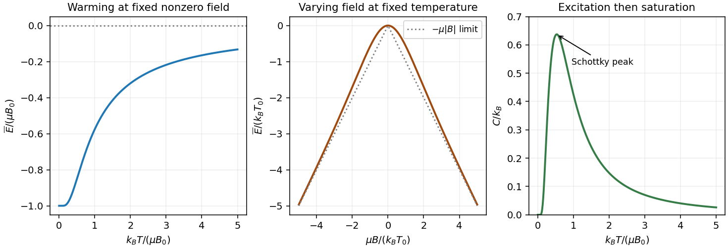
At , expanding the hyperbolic functions givesInterpreting the stated heat capacity on the same one-atom basis as the preceding calculation, its tail coefficient givesHere is used consistently with in electronvolt kelvin. For a sample of independent atoms, the total coefficient would be times the one-atom coefficient; it must first be divided by .
Finally, two derivatives of supply the second energy moment:Combining this with the heat-capacity derivative yields the canonical energy fluctuation relationIt also explains why this canonical heat capacity is nonnegative.[ref]
Past exam of the physics B course of the University of Cambridge 2014 Paper 2 Section C C11 Solution (film calculations) by Codex 0 2026-10-20
Codex 0 2026-10-20Reading the approximately straight trend in the supplied graph gives and . These are graph-read estimates, not more precise material constants. For , reversible isothermal stretching givesBoth are positive: stretching does mechanical work on the film and requires heat input to prevent cooling. Its internal energy increases by about .
Write , with . Constant then makes the reversible adiabatic conditionwhere is an arbitrary fixed reference temperature; absorbing it into the constant gives the requested logarithm convention. HenceHere . Since , integration gives . To first order this isThere is no heat exchange on this reversible adiabat. Cooling and increasing internal energy are compatible: positive area work more than offsets the decrease of the temperature-dependent energy term.
Past exam of the physics B course of the University of Cambridge 2014 Paper 2 Section C C11 Solution by Codex 0 2026-10-20
Codex 0 2026-10-20With , the thermodynamics of a liquid film givesEquality of mixed derivatives of gives the Maxwell relationUse the area convention already specified by ; do not insert an additional factor for two film faces.
Past exam of the physics B course of the University of Cambridge 2014 Paper 2 Section C C10 Solution (cycle calculations) by Codex 0 2026-10-20
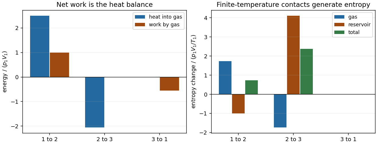
Codex 0 2026-10-20Put . For the specified ideal gas, , and . Isobaric expansion doubles temperature, so . Reversible adiabatic closure gives , henceThere is no heat input on that compression. The other stages giveTherefore andThe hot reservoir changes entropy by . The cold reservoir changes by . Since the gas completes a cycle,Although the mechanical paths can be quasistatic, heat flows across finite temperature differences in both contacts. This entropy generation explains why the efficiency is well below the Carnot value between these reservoirs.
For an isothermal final compression at , the preceding constant-volume cooling must instead end at ; keeping the old state 3 would not close the cycle. Compression then requires work , while the heat input remains . Thuswhich is lower: this isothermal compression occurs at a higher temperature throughout than the original adiabat and consumes more work. It also rejects heat during compression.
Past exam of the physics B course of the University of Cambridge 2014 Paper 2 Section C C10 Solution by Codex 0 2026-10-20
Codex 0 2026-10-20A heat engine operates cyclically, absorbing heat from a hotter source, rejecting heat to a colder sink and delivering net work . Its efficiency is . The working substance returns to its original state; the reservoirs and surroundings need not.
Past exam of the physics B course of the University of Cambridge 2014 Paper 2 Section B B9 Solution by Codex 0 2026-10-20
Codex 0 2026-10-20A central potential conserves angular momentum and confines a nonradial orbit to a plane. With reduced mass , the radial motion obeysTurning points satisfy . A radially bounded allowed interval gives bound motion, whereas an interval reaching infinity permits escape. The energy sign alone classifies these only with suitable assumptions about and barriers. Circular orbits satisfy and are radially stable when . Bound orbits in a general central potential need not close: successive periapses can precess.
For attractive inverse-square gravity, andEllipses have , , and the attracting centre at a focus; parabolic and hyperbolic escape have and . Conservation of angular momentum gives equal swept areas in equal times. The inverse-square law additionally yields . These are Kepler's laws; a harmonic central potential is another example with closed bound orbits, while generic central laws produce precession.
In a gravitational assist, a spacecraft's asymptotic speed relative to a planet is approximately unchanged but its direction turns. Transforming to the frame in which the planet has velocity givesThe spacecraft can gain or lose orbital energy; the planet supplies the compensating energy and momentum, with a very small velocity change because of its large mass.
Repulsive Coulomb scattering instead has . For incident relative kinetic energy and impact parameter , the hyperbolic orbit givesThis Rutherford scattering formula follows by equating the incident annulus to the scattered solid-angle ring. It assumes classical elastic scattering by a point Coulomb centre; screening, finite nuclear size or quantum effects can change the applicable regime.
Pinned article: Introduction to the OurBigBook Project
Welcome to the OurBigBook Project! Our goal is to create the perfect publishing platform for STEM subjects, and get university-level students to write the best free STEM tutorials ever.
Everyone is welcome to create an account and play with the site: ourbigbook.com/go/register. We belive that students themselves can write amazing tutorials, but teachers are welcome too. You can write about anything you want, it doesn't have to be STEM or even educational. Silly test content is very welcome and you won't be penalized in any way. Just keep it legal!
Intro to OurBigBook
. Source. We have two killer features:
- topics: topics group articles by different users with the same title, e.g. here is the topic for the "Fundamental Theorem of Calculus" ourbigbook.com/go/topic/fundamental-theorem-of-calculusArticles of different users are sorted by upvote within each article page. This feature is a bit like:
- a Wikipedia where each user can have their own version of each article
- a Q&A website like Stack Overflow, where multiple people can give their views on a given topic, and the best ones are sorted by upvote. Except you don't need to wait for someone to ask first, and any topic goes, no matter how narrow or broad
This feature makes it possible for readers to find better explanations of any topic created by other writers. And it allows writers to create an explanation in a place that readers might actually find it.
Figure 1. Screenshot of the "Derivative" topic page. View it live at: ourbigbook.com/go/topic/derivativeVideo 2. OurBigBook Web topics demo. Source. - local editing: you can store all your personal knowledge base content locally in a plaintext markup format that can be edited locally and published either:This way you can be sure that even if OurBigBook.com were to go down one day (which we have no plans to do as it is quite cheap to host!), your content will still be perfectly readable as a static site.
- to OurBigBook.com to get awesome multi-user features like topics and likes
- as HTML files to a static website, which you can host yourself for free on many external providers like GitHub Pages, and remain in full control

Figure 2. You can publish local OurBigBook lightweight markup files to either OurBigBook.com or as a static website.
Figure 3. Visual Studio Code extension installation.
Figure 5. . You can also edit articles on the Web editor without installing anything locally. Video 3. Edit locally and publish demo. Source. This shows editing OurBigBook Markup and publishing it using the Visual Studio Code extension. 
- Infinitely deep tables of contents:




All our software is open source and hosted at: github.com/ourbigbook/ourbigbook
Further documentation can be found at: docs.ourbigbook.com
Feel free to reach our to us for any help or suggestions: docs.ourbigbook.com/#contact