Topics (384k) Articles (398k) Users (410) Discussions (242) Comments (383) Files (13k) New article

Past papers, worked solutions and errata: www.hep.phy.cam.ac.uk/~lester/teaching/partIIIparticles/exams/index.html
The archive lists papers for 2000–2025. Worked solutions are public for 2000–2008, 2012–2018 and 2020–2025; skip those years for new solutions. The archive does not provide solutions for 2009–2011 and marks the 2019 solutions as not released publicly.
The displayed three-dimensional parabolic coordinates use and an azimuthal angle . Their coordinate tangent vectors have pairwise zero dot products, with scale factors of orthogonal coordinates and . The Jacobian determinant is . Constant or gives a family of confocal circular elliptic paraboloids; the coordinate system degenerates on the axis where . For example, fills the cap , whose rim is the unit circle and whose vertex is .
For , , and real , these orthogonal coordinates have coordinate tangents , and . Their scale factors of orthogonal coordinates are and ; the ordered Jacobian determinant is positive away from the two focal lines. Positive constant gives confocal elliptical cylinders, while generic constant gives a hyperbolic-cylinder half-branch selected by the signs of and . The limiting surface is the strip , , with arbitrary . Constant gives horizontal planes.
For a length scale , planar bipolar coordinates may be defined byThe common scale factor is , so Laplace's equation becomes away from coordinate singularities. For , constant- curves are circlesTheir radii decrease as increases; for the circle lies inside the circle. The region is therefore an eccentric circular annulus. This ordering is useful when translating coordinate boundary data into geometric language.
For a ring torus of major radius , circular torus coordinates use distance and angle in the circular cross-section, and azimuth around the central axis. The coordinate tangent vectors are the three partial derivatives of the displayed position. They are mutually orthogonal, with scale factors of orthogonal coordinates . For their ordered Jacobian determinant is , so . At the cross-section angle degenerates. These are tubular coordinates for a circular torus, rather than the confocal coordinate convention also called toroidal coordinates.
For a real conductivity tensor invariant under every rotation about a unit vector , the electric current density is . Its collinearity with a nonzero real electric field has three cases. Axial fields are always mapped to an axial current. Purely transverse fields give a collinear current exactly when , equivalently when this tensor is symmetric. Fields with nonzero axial and transverse parts require both and , making the tensor isotropic. The zero vector is included as a scalar multiple; requiring a nonzero current also requires the relevant scalar conductivity to be nonzero.
For two masses, connect each to a fixed anchor and to the other mass with equal stiffness . Set to choose units. The squared angular frequencies have characteristic equation . Requiring a frequency ratio of two means that these roots are and . Their sum and product give , yielding the two reciprocal ratios in the header. Restoring units multiplies all squared frequencies by , leaving the permitted mass ratios unchanged. The term octave refers here only to this two-to-one ratio.
For real , this differential one-form on the punctured plane is the pullback of a differential form of the nonexact angular one-form under the invertible linear transformation . It is a closed differential form for every such pair. On a region admitting a continuous complex argument, it has the local potential . In a chart with , this can be written .
There is no globally single-valued potential on the whole punctured plane. On the closed path , , , substitution gives , hence its line integral is . This contradicts the zero integral around every closed path required of an exact differential form. Around a positively oriented once-winding path the integral is . The local equation gives radial rays; away from a vertical ray its solutions as graphs are on intervals not crossing the excluded origin.
Reordering the interpolation nodes changes the successive subsets used for the divided differences and the factors of the Newton polynomial. The final interpolation polynomial remains unchanged in exact arithmetic. For , reversing gives and values . The successive divided difference columns are nowFor example, the first second divided difference is . The top row becomes , givingThe earlier partial interpolants differ because they fit different subsets: fits , whereas fits . The highest divided difference is invariant because both complete top rows finish with the same set of four interpolation nodes; this is symmetry of divided differences.
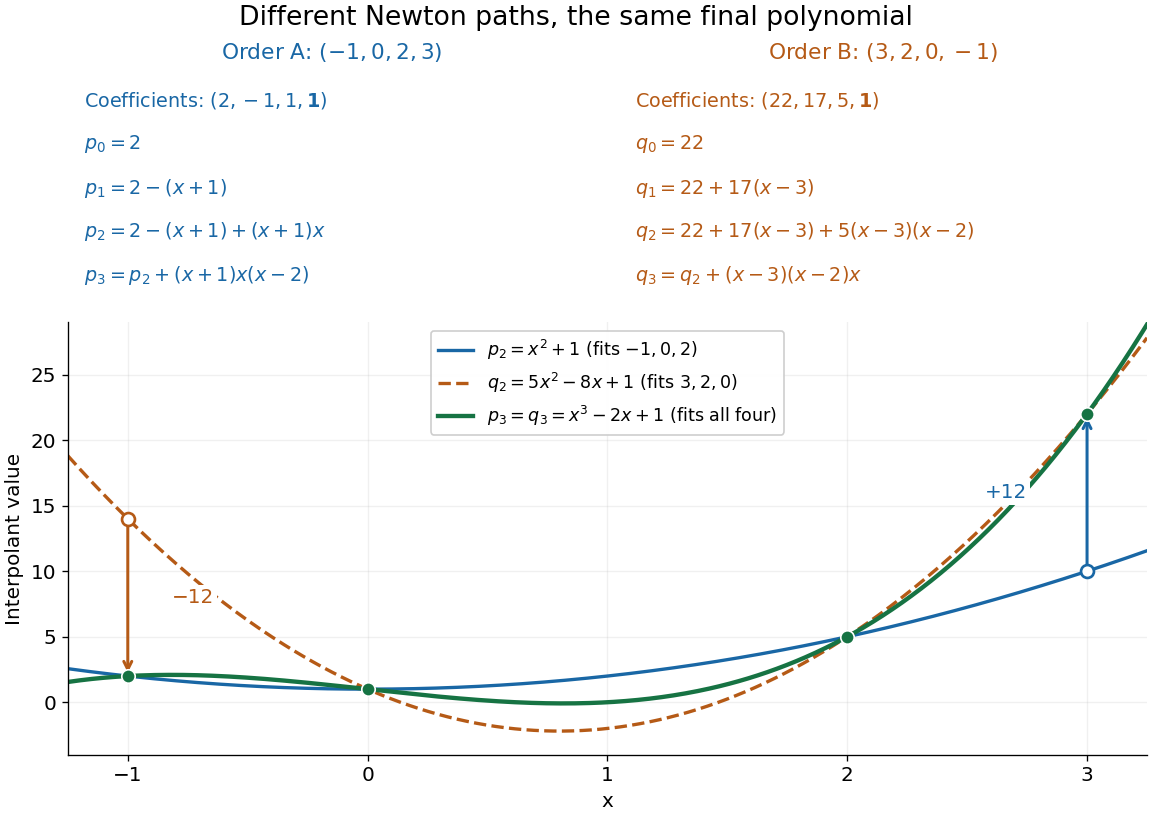
Reversing the interpolation nodes changes the Newton construction but gives the same final polynomial
. Details. This distinction is useful when checking a divided difference table: permuting all the interpolation nodes must preserve its final divided difference, even though the intermediate entries change. It also explains why data can be appended in their arrival order. In floating-point arithmetic, the subtractions and divisions may accumulate different rounding errors in different orders; exact invariance describes the mathematical polynomial, rather than guaranteeing bit-for-bit equality of numerical results.
Consider a nonrelativistic particle of mass undergoing an elastic collision with a stationary free target of mass , where . Assume the outgoing direction is uniformly distributed over solid angle in the center of mass frame; this assumption concerns the scattering angle distribution and need not hold for every target or energy. Let be the cosine of that frame's scattering angle. Transforming the outgoing velocity back to the laboratory givesThe uniform distribution of on makes uniform on . For , integration yieldsFor equal masses, take the limit : . The expected value of the fractional energy after a collision is instead . These are different averages: averaging a logarithm does not give the logarithm of an average.
For independent collisions with the same distribution, the logarithms of successive energy ratios add. ThusHere is the geometric-mean energy, and is a characteristic collision count for reaching an energy scale . It is not an exact first-passage expected value. Individual histories fluctuate, and neither the time between collisions nor absorption is specified by this model.
A material used for neutron moderation, such as water or paraffin wax in the Fermi slow-neutron activation experiment.
Choose a one-dimensional crystal with cell translation and two atoms per cell at and . Here is an intracell displacement, distinct from the interplanar spacing above. In a single-scattering approximation, a row of cells has scattering amplitudeThe sum selects reciprocal lattice positions as becomes large. At these positions, the two-site crystal basis structure factor and its squared magnitude areConsequently gives even reflections of strength and extinguishes the odd reflections. Choosing , instead gives and : the odd/even ratio is . Equal atomic numbers would not establish equal if the isotopes differ. The figure below plots these chosen coefficients, without assigning them to actual elements. Missing reflections can encode destructive wave interference within a cell, not the absence of matter at a site.
The nuclear neutron scattering length is the effective length coefficient for low-energy nuclear scattering amplitude. For the elementary coherent calculation below, use a bound coherent coefficient for each site, and neglect absorption so that is real. This coefficient describes the atomic nucleus, including its isotope and nuclear spin dependence; it is not proportional to atomic number. Replacing nuclear coefficients by electronic magnetic moments would describe a different scattering channel, with additional direction and spatial-distribution factors, as explained in magnetic neutron diffraction.
For pots per treatment and leaves per pot, the group sample mean decomposes into two averages:The variance of a sum adds the variances of the independent terms. Every pot random effect has weight , whereas each remaining error has weight , giving the short proofThis is also the variance of the arithmetic mean of the pot sample means, each with variance . Equal numbers of leaves per pot make the two averaging procedures identical.
If all leaf measurements were falsely treated as independent, the predicted variance would instead be . The ratio of correct to false variance isThus pseudoreplication can underestimate a standard error by the square root of this ratio. Equality holds when or ; sharing a pot creates an error here precisely when the shared influence has positive variance.
Choose , , and as constructed model parameters in squared length units. These are assumptions rather than fitted experimental values. For each group,The treatment contrast has expected value . Since the group errors are independent conditional on the allocation, its variance is twice the group variance, namely , whereas the false calculation gives . Its correct standard error is length units; the false value is . The variance ratio is .
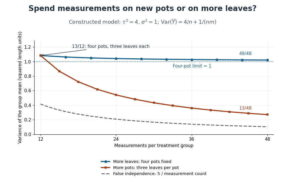
Constructed variance predictions: adding pots reduces uncertainty faster than adding leaf measurements within four pots
. Each curve uses and ; the horizontal axis counts measurements per treatment. The solid designs agree at four pots with three leaves each. The dashed curve assumes all measurements are independent and therefore illustrates pseudoreplication; none of the curves are observed experimental data. Details.With four pots fixed, increasing drives the error contribution towards zero, but the limit of the group variance remains . Measuring twelve leaves on each of four pots gives . Using the same forty-eight measurements on sixteen pots, with three leaves per pot, gives . More independent experimental units reduce both contributions. Extra nested measurements are useful for characterizing each experimental unit, but cannot average away its shared random effect. This is why sample collection effort and the number of independent treatment replicates answer different questions.[ref]
Pseudoreplication and the Design of Ecological Field Experiments by Stuart H. Hurlbert. Pseudoreplication and the Design of Ecological Field Experiments, p. 201, “Multiple samples per experimental unit”
Suppose independent Bernoulli trials give a player a win with probability , and the match ends when either player reaches wins. The player's match-win probability isFor a win with losses, the final trial must be a win. The preceding trials contain exactly wins and losses; the binomial coefficient counts their arrangements. Because , the opponent cannot already have won, and because the player has only previous wins, the match has not ended earlier. Summing the disjoint terminal events gives the formula, a truncated negative binomial distribution sum. The constant game-win probability must describe independent games, or equivalently remain the same conditional on every previous history.
In independent Bernoulli trials with success probability and failure probability , let be the trial of success and the trial of failure , for positive integers . If success occurs after failures, its final trial is a success and the preceding trials have successes and failures. The negative binomial stopping argument therefore gives the title sum.
Put . By trial , at least one target must have been reached, so the same event is that a binomial distribution with trials has at least successes. Conditioning instead on the final trial of a block of trials givesIndeed, more than successes in the full block guarantee the success target won; with exactly successes it won only when the final trial was a failure. These disjoint cases explain the extra boundary term. A zero success target wins immediately; a zero failure target has already been reached. To include in the displayed finite sum requires the explicit generalized convention ; an upper summation limit of denotes an empty sum.
Pinned article: Introduction to the OurBigBook Project
Welcome to the OurBigBook Project! Our goal is to create the perfect publishing platform for STEM subjects, and get university-level students to write the best free STEM tutorials ever.
Everyone is welcome to create an account and play with the site: ourbigbook.com/go/register. We belive that students themselves can write amazing tutorials, but teachers are welcome too. You can write about anything you want, it doesn't have to be STEM or even educational. Silly test content is very welcome and you won't be penalized in any way. Just keep it legal!
Intro to OurBigBook
. Source. We have two killer features:
- topics: topics group articles by different users with the same title, e.g. here is the topic for the "Fundamental Theorem of Calculus" ourbigbook.com/go/topic/fundamental-theorem-of-calculusArticles of different users are sorted by upvote within each article page. This feature is a bit like:
- a Wikipedia where each user can have their own version of each article
- a Q&A website like Stack Overflow, where multiple people can give their views on a given topic, and the best ones are sorted by upvote. Except you don't need to wait for someone to ask first, and any topic goes, no matter how narrow or broad
This feature makes it possible for readers to find better explanations of any topic created by other writers. And it allows writers to create an explanation in a place that readers might actually find it.
Figure 1. Screenshot of the "Derivative" topic page. View it live at: ourbigbook.com/go/topic/derivativeVideo 2. OurBigBook Web topics demo. Source. - local editing: you can store all your personal knowledge base content locally in a plaintext markup format that can be edited locally and published either:This way you can be sure that even if OurBigBook.com were to go down one day (which we have no plans to do as it is quite cheap to host!), your content will still be perfectly readable as a static site.
- to OurBigBook.com to get awesome multi-user features like topics and likes
- as HTML files to a static website, which you can host yourself for free on many external providers like GitHub Pages, and remain in full control

Figure 2. You can publish local OurBigBook lightweight markup files to either OurBigBook.com or as a static website.
Figure 3. Visual Studio Code extension installation.
Figure 5. . You can also edit articles on the Web editor without installing anything locally. Video 3. Edit locally and publish demo. Source. This shows editing OurBigBook Markup and publishing it using the Visual Studio Code extension. 
- Infinitely deep tables of contents:




All our software is open source and hosted at: github.com/ourbigbook/ourbigbook
Further documentation can be found at: docs.ourbigbook.com
Feel free to reach our to us for any help or suggestions: docs.ourbigbook.com/#contact