Topics (384k) Articles (398k) Users (410) Discussions (242) Comments (383) Files (13k) New article
A plane shock moving at speed through initially stationary gas has upstream speed and downstream speed in the shock frame, where is the shock compression ratio. Transforming back to the initial slab frame gives . At the breakout time , a uniform downstream slab has thickness . The strong monatomic limit has , hence and . This uses a maintained planar post-shock state; boundary rarefactions and variations of shock speed can change the actual thickness of a freely evolving finite cloud.
Define and, elsewhere,All first and second partial derivatives exist at the origin: and . Thus its Hessian matrix there is the positive-definite matrix . Nevertheless and for , so the origin is a saddle point of a scalar function. A valid second-derivative test needs a second-order Taylor expansion with a remainder ; continuous second partial derivatives in a neighborhood are a sufficient hypothesis. Existence of those derivatives at the point alone does not supply this hypothesis.
Here is a short proof that uses only the row space. For a vector subspace , let be the dimension of its projection map onto the first coordinates, with . In any reduced row echelon form with row space , counts the pivot columns among those first columns: later-pivot rows project to zero, while earlier-pivot rows remain linearly independent. Thus the positions where determine all pivot positions from alone.
If those positions are , the map sending to is an isomorphism : the reduced nonzero rows map to the standard basis. Its th row is therefore the unique vector of with pivot-coordinate values equal to the th standard basis vector. Any other reduced row echelon form with that row space has identical nonzero rows in identical order. At a fixed matrix size, the remaining rows must be zero. Together with existence by Gaussian elimination, this proves uniqueness.
For row reduction with a parameterized right-hand side at , the nonzero reduced equations areColumn 3 has no pivot element, so is a free variable in a linear system. Taking gives every solution:There is no further restriction on . Independent substitution into the original linear system givesConversely, the two reduced equations force exactly these coordinate formulas, so no solutions have been omitted. The same computation with zero right-hand side gives the kernel . Its dimension is one. The rank-nullity theorem appears here as : two pivot columns and one freely chosen coordinate account for the three unknowns.[ref]
The Rank Theorem. Interactive Linear Algebra by Dan Margalit and others; §2.9, Rank Theorem and preceding pivot-column/free-variable count
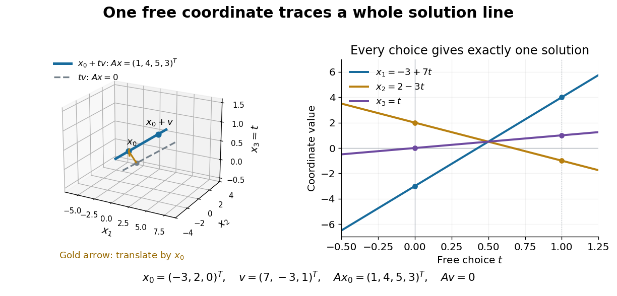
One free variable in a linear system traces an affine solution space of a linear equation parallel to its kernel
. Details. In general a consistent linear system has solution set . Subtracting from proves this description in both directions. The particular solution places the affine subspace, and the kernel supplies its directions.[ref]
Solution Sets. Interactive Linear Algebra by Dan Margalit and others; §2.4.2, Key Observation and its proof: translate homogeneous solutions by any particular solution
Over the real numbers this example is an entire line; over the rational numbers the same formula uses rational . A free variable in a linear system over a finite field instead has only finitely many choices.The pivot columns identify a different object: the original column space. Here they selectwhich form its basis, while . The corresponding reduced columns are and ; their linear span is a different plane. For example, every original output satisfies , but does not. Since is an invertible matrix, column linear relations survive even though the output vectors move. This is why choosing original columns at the reduced pivot positions works.
Reciprocal lattice change in a structural phase transition by  Codex 0 Created 2026-10-18 Updated 2026-10-20
The reciprocal lattice of a body-centered cubic lattice is face-centred cubic, and that of a face-centered cubic lattice is body-centred cubic. In both cases its conventional cubic side is if the direct conventional side is . Thus a direct BCC-to-FCC phase transition reverses the reciprocal lattice types. The reciprocal primitive cell volume is , so thermal expansion contracts reciprocal spacings, while a discontinuous change in direct primitive unit cell volume gives an inverse change in reciprocal cell volume.
A first-order structural transition need not continuously deform one perfect reciprocal array into another. Phase coexistence, new orientation variants, domains and loss of single-crystal alignment can produce two sets of diffraction peaks or many differently oriented sets. The two endpoint lattice types alone do not specify the transformation path or orientation relationship.
For a simple random walk on an infinite regular tree of degree , every vertex other than the chosen root has one neighbour closer to the root and farther away. The graph distance from the root is therefore a nearest-neighbour Markov chain on the nonnegative integers, with the displayed bulk transition probabilities and a certain outward step from zero. For shell probabilities ,Shell probabilities include all vertices at the given distance. They differ from single-vertex probabilities by the shell size, at the root and for .
Past exam of the quantum condensed matter course of the University of Cambridge by Codex 0 2026-10-18
Codex 0 2026-10-18Past-paper archive: www.sp.phy.cam.ac.uk/drp2/home. The archive lists papers for 2004–2018; worked solutions for these exams have not been verified. Lecture-problem solutions are not treated as past-exam solutions.
The binary-pulsar Einstein delay is the periodic clock-rate contribution to pulse arrival times from a pulsar moving in an eccentric binary. Near closest approach, the pulsar's orbital speed is larger and the companion's gravitational potential is deeper. Time dilation and gravitational redshift therefore make its clock run at a different rate relative to a distant time coordinate.
At leading order the variable timing term is , with eccentric anomaly and time amplitude . Constant clock-rate offsets are absorbed into the fitted pulsar spin. This term is distinct from the geometric binary-pulsar Roemer delay and the propagation Shapiro time delay. Fitting it with other orbital observables constrains the component masses and tests general relativity.[ref]
Binary Pulsars and Relativistic Gravity by Joseph Hooton Taylor Jr.. Section III, Model Fitting: relativistic time transformation and post-Keplerian timing parameters
The difference between an observed arrival time and its model prediction. Positive pulsar timing residuals mean late arrivals in this convention. A periodic residual can expose an omitted orbit; a smooth long-term residual can also come from a wrong spin model or clock correction. Fitting and checking alternative causes are part of the inference, rather than interpreting every residual as gravitational radiation.
Pulsar dedispersion aligns radio wave arrival times in separate frequency channels before combining them. For an original illustrative model chooseBoth bracketed ratios are dimensionless, so supplies all the time units. The reference is : delays are there, at , and at . These are chosen model values, not measurements of the first pulsar. Subtracting the delay aligns the peaks; summing channels first spreads a short pulse over a longer interval and reduces its peak. Finite channel width and incorrect delay parameters leave residual smearing.
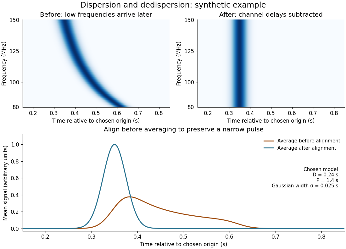
The integrated electron number density along the line of sight, conventionally quoted in . A dispersion measure is a column, not a unique distance: converting it into distance requires a model of the interstellar medium. A clumpy nearby column and a longer dilute column can give the same pulsar dispersion delay.
For fixed strict preferences, the same output of the Gale-Shapley algorithm gives each receiver its worst partner obtainable in any stable matching, treating unmatched as last. "Worst" is restricted to stable possibilities: a receiver might still receive its favourite acceptable partner if every stable matching assigns it that partner. Reversing the proposing side gives receivers their best stable partners instead.
For a short proof, let be a proposer-optimal stable matching and any other stable matching. If a receiver preferred to , then proposer optimality would make prefer to , since the partners differ and preferences are strict. The pair would block . Therefore no receiver prefers its partner in to its partner in . In the worked example, right-side ranks in are for , whereas gives them . Neither outcome is universally best for both sides.
For a random variable with probability density function on an interval, let , where is a diffeomorphism onto another interval. The change of variables formula givesIndeed, integrating the right-hand side over an outcome interval gives the probability that lies in its inverse image. The absolute derivative preserves positive probability when reverses orientation. A gravity deflection of an atomic beam is a physical example: its speed-to-height transformation changes the probability density and its mode.
Columbia University's institutional laboratory manual, Experiment 1, Glassware Calibration, Primary and Secondary Standards, and Manual Titrations, Part 3, specifies two weighed – portions of potassium hydrogen phthalate, transferred completely into separate Erlenmeyer flasks. Dissolve each in approximately distilled water; any warmed sample cools to room temperature before titration. Add two or three drops of phenolphthalein. Rinse and condition a clamped burette with the diluted sodium hydroxide, then titrate while swirling to faint pink lasting about seconds. Calculate concentration from each portion's own mass and delivered titre; repeat if results scatter. Part 1 identifies a Mettler balance, and Part 2 includes paired weighings of exposed sodium hydroxide and potassium hydrogen phthalate. These are prescribed procedures, not reported measurements.[ref]
The same manual directs keeping the diluted sodium hydroxide covered and limiting air exposure after titrant standardization.[ref]
Glassware Calibration, Primary and Secondary Standards, and Manual Titrations, Columbia University Experiment 1. Experiment 1, Part 3, introductory paragraph and step 1
The MIT handout explains the associated carbon dioxide problem: carbonate contamination of sodium hydroxide is controlled during preparation, bottles are promptly capped, and atmospheric carbon dioxide makes the pink phenolphthalein endpoint fade.[ref]The Potentiometric Titration of an Acid Mixture (MIT 5.310 laboratory handout). Printed Titration-5, §IV.1 and footnote 3; Titration-6, footnote 6
Consequently, a standardized concentration applies to the stored chemical solution under its handling conditions; continued uptake of carbon dioxide can change the reacting inventory per delivered volume.The color is the readout, and stoichiometry supplies the inference. Phenolphthalein indicates a pH range, so its first reproducible pale pink is an operational titration endpoint, rather than a direct observation of equal reacting inventories. A potentiometric titration can locate an endpoint from a pH versus volume curve, but glass electrode calibration alone still does not determine sodium hydroxide concentration. Repeat portions test scatter; incomplete dissolution, an unmatched titration blank, or a shared endpoint error can bias all repeats together.
Let be the transferred sample mass, the known mass fraction of the intended chemical compound, and its molar mass. In a model with complete dissolution and chemically inactive impurities,The purity fraction is dimensionless: would mean , not . These equations assume that the impurity contributes no titrant demand; an impurity that also reacts needs its own inventory equation. The value of must refer to the same preparation state as , for example the specified dry material. A mass fraction assigned before unaccounted uptake of water cannot simply be used after it.
For an original worked example, stipulate pure potassium hydrogen phthalate, abbreviated KHP, so , a selected mass , and rounded molar mass . The NIST Chemistry WebBook lists formula and molecular weight , consistent with the rounded molar mass used here.[ref]
potassium hydrogen phthalate. NIST Chemistry WebBook, SRD 69, potassium hydrogen phthalate, CAS 877-24-7; Formula and Molecular weight fields
The selected mass, purity assumption and volumes in this example are chosen inputs, not measured results or a claim about a real batch's purity.The acid-bearing anion of potassium hydrogen phthalate loses one proton to hydroxide. The net chemical equation isThus sodium hydroxide has one-to-one stoichiometry with potassium hydrogen phthalate in this neutralization, givingChoose a delivered endpoint titre of and matched titration blank of . ThenThe extra displayed digits show the arithmetic of the stipulated model; they do not establish experimental accuracy. A compact rounded result is .
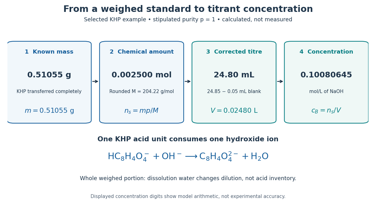
A primary standard connects known mass to amount of substance, corrected titre, and titrant concentration
. Original calculated inventory diagram for selected potassium hydrogen phthalate, stipulated , rounded molar mass , and one-to-one sodium hydroxide neutralization. The endpoint and matched titration blank are chosen examples, not observations. Details.When the entire weighed portion is titrated, added water changes concentration and the pH path but preserves the initial acid inventory. The dissolution volume therefore does not appear in . If instead a volumetric flask prepares a stock and a volumetric pipette selects an aliquot, the selected inventory is for homogeneous stock, with delivered aliquot volume and final stock volume . The same bookkeeping explains why complete transfer matters even when the amount of dissolution water is approximate.
A resistance pressure gauge is a pressure sensor whose electrical resistance is calibrated against pressure. Even a simple local response needs both pressure and temperature. For an original illustrative model definewhere is the reference electrical resistance at , , and zero history offset. The derivatives and are local sensitivities with units and , respectively; is a dimensionless history offset. Constant sensitivities are an approximation over a chosen range, not material constants valid at every pressure.
Choose synthetic coefficients and , with and . A measured ratio then gives . Ignoring the temperature change gives , a error. This model is deliberately stipulated; these numbers are not measured manganin coefficients or Bridgman's data.
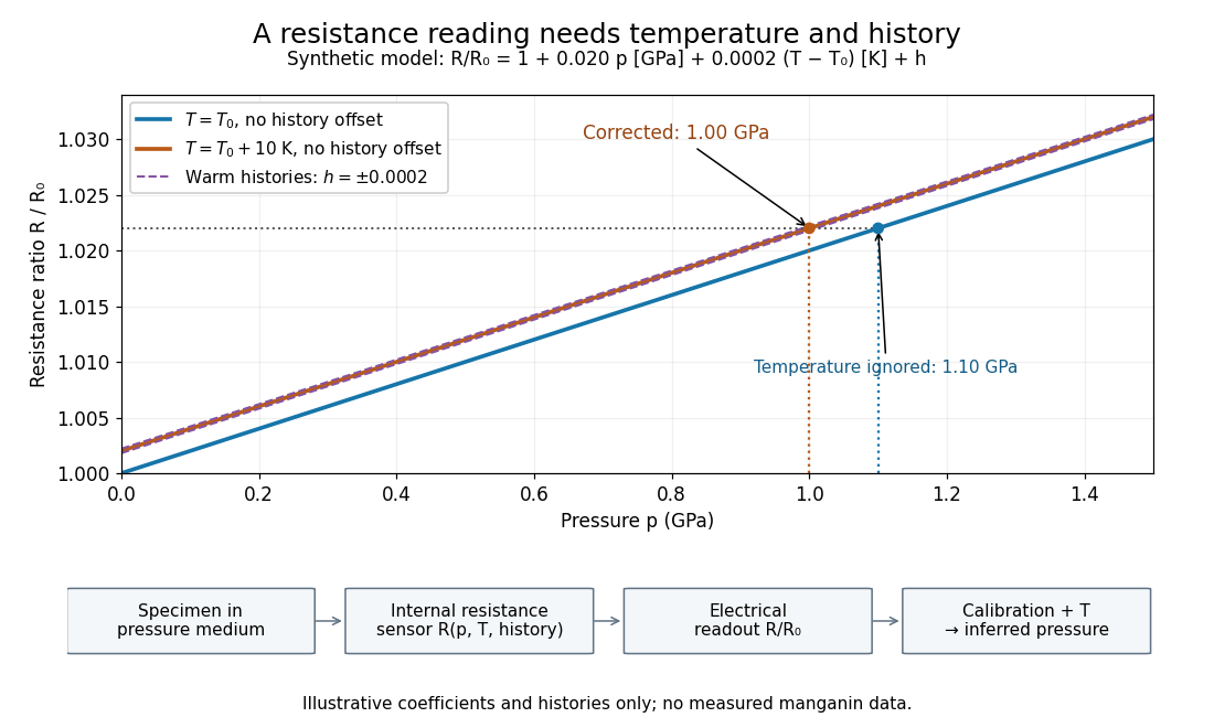
Pressure calibration: a synthetic electrical resistance response with temperature and hysteresis offsets
. Original calculated example. The blue reference line has , ; the orange line has , . Dashed lines illustrate two histories with , not observed data. A ratio 1.022 maps to 1.00 GPa after correcting temperature, or 1.10 GPa if read against the blue line. The lower chain distinguishes the specimen, the internal sensor, the electrical readout and the calibrated pressure. Details.If two histories differ by , their outputs at the same pressure differ by ; interpreting both with a single history-free curve gives an apparent pressure separation . The half separation is . Reversing the drive can additionally cause mechanical friction hysteresis, independently of this sensor model. Record both the electrical calibration history and the loading direction.
For independent small standard measurement uncertainties and exact stipulated , first-order propagation givesFor , , and , this is . Real calibration also includes coefficient measurement uncertainties, correlations, reference-point measurement uncertainty, and any unresolved nonhydrostatic loading. A sensor calibrates its local environment; it cannot by itself certify the absence of deviatoric stress throughout the sample.
For polar coordinates , with , the Jacobian determinant is . The change of variables formula therefore gives the area element . Integrating over the radial interval gives per unit angle. Bounds must describe the intended region without counting it more than once.
For boundary value on and zero outside, integrating the Poisson kernel for the upper half-plane gives the displayed bounded harmonic function for . It approaches the assigned values at boundary continuity points and the midpoint value at either jump. Changing the value at an isolated endpoint does not alter the integral. This is the unique bounded harmonic extension; pointwise decay in the vertical direction alone, without a spatial growth restriction, does not give uniqueness.
Consider an ideal pressure-driven closure plug with a large chamber-facing projected area . Its opposite side seats against a smaller annular packing surface area . The remaining projected part is the unsupported area: it has no opposing packing contact in that plane. Here is the chamber pressure relative to the exterior. Let denote the mean axial compressive contact stress on the packing, not the chamber's hydrostatic stress.
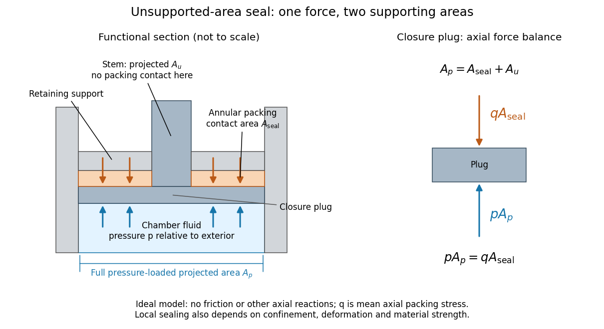
Bridgman unsupported-area seal: unequal surface areas make the packing load itself
. Original functional section and force diagram, with no historical dimensions. Chamber pressure acts over ; the packing reaction acts over the smaller . The central stem occupies the unsupported projected part . Blue arrows show the chamber load on the closure; orange arrows show the opposing packing reaction. The drive piston that pressurizes the chamber is a separate experimental function. Details.Neglect friction, the plug's weight, and other axial reactions. The plug's Newton's second law in static balance isThe load is the same on both sides; its smaller supporting surface area raises the packing's mean contact stress. For a stipulated ratio and , the ideal seating stress is . Its excess over chamber pressure is . Reducing to zero removes this amplification. This is the elementary force balance behind self-energizing seating, consistent with the lecture's Figure 1 caption.[ref]
The relation is a model, not a universal sealing law. The mean axial contact stress need not equal the local contact stress along every possible leakage path. Confinement and plasticity in continuum mechanics determine whether the packing closes a gap or instead extrudes into it. Friction diverts load into other surfaces; material plasticity in continuum mechanics changes contact geometry; the vessel must carry its own stress. A finite initial seating load may also be needed before chamber pressure can develop. An arbitrarily small does not yield arbitrarily useful sealing: the assumptions fail when local deformation, extrusion or structural failure takes over.
Pinned article: Introduction to the OurBigBook Project
Welcome to the OurBigBook Project! Our goal is to create the perfect publishing platform for STEM subjects, and get university-level students to write the best free STEM tutorials ever.
Everyone is welcome to create an account and play with the site: ourbigbook.com/go/register. We belive that students themselves can write amazing tutorials, but teachers are welcome too. You can write about anything you want, it doesn't have to be STEM or even educational. Silly test content is very welcome and you won't be penalized in any way. Just keep it legal!
Intro to OurBigBook
. Source. We have two killer features:
- topics: topics group articles by different users with the same title, e.g. here is the topic for the "Fundamental Theorem of Calculus" ourbigbook.com/go/topic/fundamental-theorem-of-calculusArticles of different users are sorted by upvote within each article page. This feature is a bit like:
- a Wikipedia where each user can have their own version of each article
- a Q&A website like Stack Overflow, where multiple people can give their views on a given topic, and the best ones are sorted by upvote. Except you don't need to wait for someone to ask first, and any topic goes, no matter how narrow or broad
This feature makes it possible for readers to find better explanations of any topic created by other writers. And it allows writers to create an explanation in a place that readers might actually find it.
Figure 1. Screenshot of the "Derivative" topic page. View it live at: ourbigbook.com/go/topic/derivativeVideo 2. OurBigBook Web topics demo. Source. - local editing: you can store all your personal knowledge base content locally in a plaintext markup format that can be edited locally and published either:This way you can be sure that even if OurBigBook.com were to go down one day (which we have no plans to do as it is quite cheap to host!), your content will still be perfectly readable as a static site.
- to OurBigBook.com to get awesome multi-user features like topics and likes
- as HTML files to a static website, which you can host yourself for free on many external providers like GitHub Pages, and remain in full control

Figure 2. You can publish local OurBigBook lightweight markup files to either OurBigBook.com or as a static website.
Figure 3. Visual Studio Code extension installation.
Figure 5. . You can also edit articles on the Web editor without installing anything locally. Video 3. Edit locally and publish demo. Source. This shows editing OurBigBook Markup and publishing it using the Visual Studio Code extension. 
- Infinitely deep tables of contents:




All our software is open source and hosted at: github.com/ourbigbook/ourbigbook
Further documentation can be found at: docs.ourbigbook.com
Feel free to reach our to us for any help or suggestions: docs.ourbigbook.com/#contact