Topics (384k) Articles (398k) Users (410) Discussions (242) Comments (383) Files (13k) New article
The natural logarithm has the parameter-integral representationFor , the identity shows convergence: the absolute value is at most , which is integrable when . At , the apparent singularity is removable, with limiting value .
Write the left side as . On a compact parameter interval with , its differentiated integrand is bounded by the integrable function . The dominated convergence theorem justifies differentiation under the integral sign, giving . Since , the fundamental theorem of calculus gives . At , the original improper integral diverges as , and it also diverges for .
Integrating the geometric series for from zero to gives the displayed power series for . It has radius of convergence one. At the alternating series test gives conditional convergence to ; at the negative harmonic series diverges. Replacing by gives . An expression formed by substituting a nonlinear function for need not have the same convergence range after it is re-expanded as a Taylor series in the new variable.
Albert Abraham Michelson's 1907 lecture, Recent Advances in Spectroscopy, pp. 171–172, connects counting interference fringes with a reproducible length standard. Broad or multiple spectral lines obscured fringes at large path differences; red cadmium emission supplied a suitable source. His 1907 Nobel Prize in Physics recognized optical precision instruments and their spectroscopy and metrology applications.[ref]
Recent Advances in Spectroscopy by Albert Abraham Michelson. Nobel Lectures, Physics 1901–1921; Michelson, Nobel lecture, printed pp. 171–172; official prize motivation, printed p. 158
His authored account of the metre comparison at Sèvres describes a heated, evacuated cadmium discharge tube and a spectrometer selecting one spectral line. A movable reference mirror was compared with pairs of silvered parallel surfaces defining intermediate standards. Counted interference fringes established a short interval; repeated comparisons extended it to a decimetre and then a metre. White-light fringes located surface coincidence, while monochromatic fringes supplied counts and fractional orders. A thermally shielding box, firm pier, calibrated translation screw and tested thermometers controlled drafts, vibration, travel and temperature. Uniform temperature mattered in comparisons; the final standard required an absolute temperature reading. Optical microscopes made the final comparison to the marked metre bar, limiting the whole result.[ref]
Lecture V: Light Waves as Standards of Length. Michelson, Light Waves and Their Uses (1903), Lecture V, Figs. 70–77: intermediate standards, counting, temperature controls and final microscope comparison
This is a measurement chain, rather than one enormous unchecked fringe count: short intervals establish whole orders; fractional-order readings refine each longer comparison. The optical coherence envelope helps locate white-light coincidence, whereas the carrier phase difference measures small departures from it. Repetition checks counting mistakes, but agreement alone cannot exclude shared systematic errors. The general lesson of metrology is to preserve the link from the optical ruler through each transfer and control to the final length.
Precision displacement measurement with a Michelson interferometer by  Codex 0 Created 2026-10-18 Updated 2026-10-20
A Michelson interferometer turns displacement into a count of interference fringes: a moving mirror changes both the outward and return paths. This lets a wavelength act as a ruler whose divisions need no engraving. Assume normal incidence, a fixed reference arm, stable refractive index along the moving arm, and fixed vacuum wavelength . Write for the wavelength in that medium and take positive away from the beam splitter. The change in optical path difference, the accumulated phase difference, and the signed number of complete interference fringe cycles areThe factor two comes from propagation geometry: moving the mirror by adds before reflection and afterward. One bright-to-bright cycle means mirror travel ; bright-to-dark means , half a cycle. All lengths must use compatible units, and is dimensionless. A constant reflection phase difference changes the initial fringe position but cancels from this change formula.
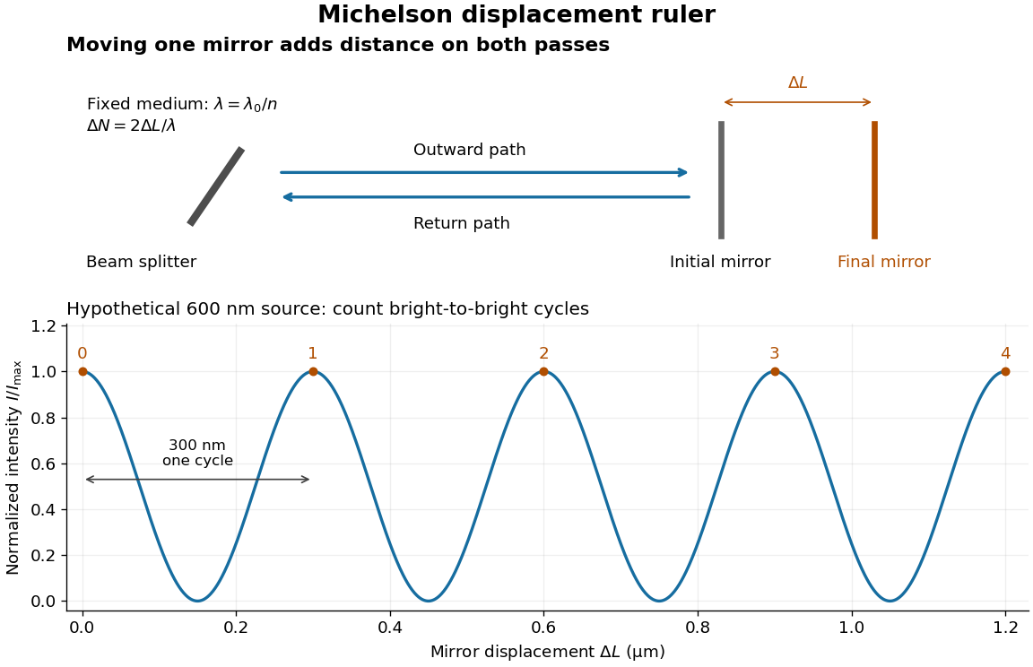
Mirror displacement, doubled optical path difference, and counted interference fringes for a hypothetical Michelson interferometer
. Details. For an original hypothetical example, suppose in the actual surrounding medium and a continuous scan gives cycles, including the final fractional cycle. Then . With the wavelength treated as exact, a fringe-reading measurement uncertainty of cycle contributes to the displacement measurement uncertainty. An uncertainty of in a local phase difference instead corresponds to . This illustrates measurement resolution, not a complete claim of accuracy: wavelength calibration, air changes, mirror tilt and missed cycles can dominate.
To separate the oscillating readout from its optical coherence envelope, use the local modelHere is detected light intensity, is the mean level, is a fixed bias wave phase, and is interferometric visibility. A fine scan of measures the carrier phase difference; a coarse scan can map the temporal optical coherence envelope through . The envelope maximum locates matched delays only under the source and apparatus assumptions; it is not a bright fringe identifying an arbitrary mirror position. Even with known , one intensity reading leaves the cosine sign and whole-cycle ambiguities. Continuous motion of known direction, or an independently obtained pair of signals in phase quadrature, is needed to recover signed travel through reversals.
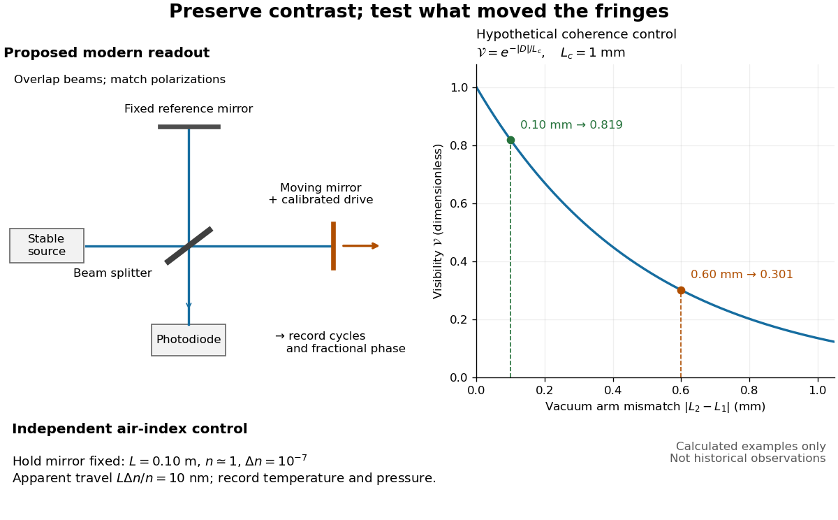
Proposed Michelson interferometer readout and hypothetical optical coherence and refractive index controls
. Details. The figure's original control example stipulates equal arm light intensities, matching linear polarizations, and a Lorentzian optical spectrum giving with . In vacuum, arm mismatches and give and . Matching the arms improves the phase difference readout without changing its travel per cycle. A fine mirror scan of one cycle changes by only for the stipulated source, much less than . These are calculated values, not historical data.
A proposed measurement sequence follows from this model. Overlap the returning beams, match their linear polarizations, find a high-contrast delay and use a small calibrated mirror scan to determine the sign and fringe period. Read a fixed spatial sample of the interference fringes with a photodiode; record each arm separately and the dark signal, avoid detector saturation, and retain enough time resolution to count every cycle. Approach mechanical settings consistently and repeat the return scan to expose lost motion or drift. For very small changes, bias near phase quadrature, where is largest; an intensity extremum has zero first-order sensitivity. A known drive voltage alone does not provide measurement calibration for mirror travel: compare the actual travel with the fringe count using an independently known wavelength.
Control temperature, pressure, vibration and air currents because the instrument measures optical path difference, not mirror motion alone. For a fixed reference arm and fixed , the first-order change of the moving arm's round-trip path is . Thus an unrecognized mimics . A hypothetical , , and give apparent travel. Holding the mirror still while varying or monitoring the air conditions tests this confounder. Separate checks of alignment, wavelength stability and thermal expansion are necessary before sub-fringe measurement resolution becomes a defensible measurement uncertainty.
Matrix powers for a diagonalizable matrix with two eigenvalues by Codex 0 Created 2026-10-18 Updated 2026-11-05
Codex 0 Created 2026-10-18 Updated 2026-11-05If a diagonalizable matrix has distinct eigenvalues , its spectral projections of a diagonalizable matrix are and . Raising the diagonal form to a nonnegative integer power gives the displayed formula. Equivalently, interpolate the scalar function by a degree-one polynomial at , then apply it to . The diagonalizability assumption matters: knowledge of two eigenvalues alone does not exclude nontrivial Jordan blocks.
A diagonal matrix entry uses the same row and column index. The diagonal entries of a lower triangular matrix determine its determinant by their product.
A device with a reference magnetic layer whose magnetization is comparatively fixed and another layer whose magnetization responds more readily to an applied field. The resistance reads their relative alignment. Fert's account describes how such giant magnetoresistance sensors entered hard-disk read heads in 1997.[ref]
Nobel Lecture: Origin, development, and future of spintronics by Albert Fert. p.1519, spin-valve structure and historical read-head adoption
Giant magnetoresistance connects the relative magnetizations of adjacent magnetic layers to their electrical transport. In a suitable magnetic-metal/nonmagnetic-metal stack, aligning the layers can leave one spin channel with an easy conducting path through both magnetic layers; opposite alignments make each channel encounter a more resistive layer. Albert Fert's account traces the spin-dependent-conduction idea to Nevill Mott and distinguishes the later device geometries.[ref]
Nobel Lecture: Origin, development, and future of spintronics by Albert Fert. pp.1517–1520, spin-dependent conduction and CIP/CPP geometry
The beauty is that a magnetic arrangement becomes an electrical readout. Preparing reproducible layers, establishing their magnetizations, and measuring electrical resistance are separate parts of that inference. The Fe-Cr giant magnetoresistance experiments show how those parts were joined; the two-current resistor model isolates a simple transport mechanism under stated assumptions.
Consider isotropic electrons and electron holes with equal density , charges , equal positive charge carrier mobility , and single-species zero-field electrical conductivity . In a transverse magnetic field, opposite Hall conductivity components cancel, while diagonal components add to . Inverting gives and . Its large-field growth is . The total zero-field resistivity is , half the single-species resistivity; confusing these quantities introduces a factor-of-two normalization error.
If one temperature-dependent relaxation scale controls a fixed carrier population and fixed orbital geometry, the magnetoresistance ratio can collapse onto a function of . This is Kohler's rule. For the equal-mobility compensated two-carrier magnetoresistance model, and . Therefore plotting against gives a common straight line of slope . A collapse tests the scaling relation; it does not by itself prove this particular microscopic carrier model. Multiple independently varying scattering times or carrier populations can spoil it.
The Anderson positron track experiment identified a light positively charged particle, now called the Positron, by combining magnetic bending, loss of kinetic energy in lead, and particle range. Each observation answered a different question: bending constrained momentum, the lead supplied a direction of travel, and particle range tested the proposed mass.
Carl David Anderson's The Positive Electron (1933), pp. 491–493, describes the 1932 discovery in a vertical cloud chamber with a magnetic field. A lead plate separated two photographed track segments. The effective viewing depth was along the magnetic field, with transverse diameter: this restricted out-of-plane motion. The photographic readout supplied curvature on both sides. Comparisons with electron tracks under the same conditions constrained ionization; specific ionization was not directly measured for these events. He tested accidental alignment of unrelated tracks and rejected a reversed electron interpretation requiring an increase of kinetic energy in lead. Assuming unit electric charge, the mass bound was about twenty electron masses, rather than an exact mass determination. The paper credits Robert Andrews Millikan with the design and Seth Henry Neddermeyer with assistance.[ref]
The Positive Electron by Carl David Anderson. pp. 491–493, Fig. 1 and charge/mass discussion; p. 494, acknowledgment
Preparation used rapid piston expansion and a water–alcohol mixture in the cloud chamber; cooling permitted droplets to form along ionization trails. A camera photographed these droplets. Initially, expansions occurred at random, so many photographs contained no tracks. Later counter triggering improved the useful yield.[ref]
Carl David Anderson by William Hayward Pickering. Biographical Memoirs: Volume 73; William H. Pickering, Carl David Anderson, pp. 27–28: preparation, photographs and timing
In The Production and Properties of Positrons, his 1936 lecture, Carl David Anderson describes the chamber inside an electromagnet and explains why the lead plate was decisive: after losing kinetic energy, a particle bent more sharply. He describes a proton hypothesis predicting only of particle range, against an observed path longer than . These are historical values from the lecture, not the stipulated example below. The point was the incompatibility of particle range with the momentum inferred from curvature, rather than positive electric charge alone.[ref]
The Production and Properties of Positrons by Carl David Anderson. Nobel Lectures, Physics 1922–1941; pp. 365–366, electromagnet, lead-plate direction test and proton range comparison
Consider lab-neutral parallel wires with stationary positive line density and electron line density . Let wire 1's electrons move at along the wire and wire 2's at . The conventional currents are . In the rest frame of wire 2's electrons, wire 1's transformed total linear charge density is . Its radial electric field is .
A wire-2 electron at rest there feels only an electric force. Transforming its transverse force back to the lab divides it by , and multiplying by the lab electron count per length giveswith positive radial direction away from wire 1. The lab-stationary positive charges feel zero net electric force because wire 1 is neutral in their frame. Equal current directions attract; opposite directions repel. Transforming force on each carrier and then counting carriers in the specified frame avoids an incorrect extra length-contraction factor in force per unit length.
In the plane wave basis of a ring, has matrix elements . Near , degenerate perturbation theory on givesup to corrections from remote states. Thus the avoided crossing gap is to first order when .
For , a parabolic approximation about a potential minimum instead gives a local quantum harmonic oscillator spacing . A local gauge transformation removes the flux from this approximation. Actual ring levels retain exponentially small flux dependence through quantum tunnelling, while nonquadratic corrections to their mean energies are algebraic in .
For reversible quasistatic magnetic circuits with flux linkages , currents and mechanical coordinate , write . The Legendre transform obeys . Thus , while . In a linear reciprocal system numerically, but the variables held fixed in their force derivatives differ. The coenergy formulation includes the effect of electrical sources maintaining the currents; it avoids reversing the sign of the magnetic force by differentiating stored energy under the wrong constraint.
Spatial variations in energy, including crystal defects, can trap a magnetic domain wall. This is magnetic domain-wall pinning. Increasing the applied magnetic field can release the wall into a collective jump.
Prepare two uniform specimens with the same material, direction and , but different deforming lengths . Keep grip engagement, adapters, loading window and measurement configuration equivalent. Determine separately by linear regression with its own displacement intercept. Subtracting the two series equations eliminates the common machine compliance:This is an inverse problem: one length supplies only one equation for two unknowns, while two distinct lengths separate the length-dependent specimen contribution from the constant contribution. In a graph of compliance against length, the slope is and the vertical intercept is . It is the compliance, not , that is linear in .
The dimensional analysis is revealing: , so . For , the ideal model requires . A negative fitted challenges the common-intercept assumptions or the measurements. Two lengths determine two parameters exactly, so they cannot test the assumed straight line; three or more lengths allow regression residuals to reveal departures. Nearly equal lengths amplify slope errors through the small difference . If the actual apparatus compliances differ by , the inferred length slope becomes .
A logical implication holds whenever its premise is false. For partial correctness, an execution that never terminates supplies no final state violating the postcondition.
A log-log plot uses logarithmic scales on both axes. For a positive power law with , positive references giveIts transformed slope is the exponent when both axes use the same logarithm base and the slope is measured in logarithmic coordinate units. For example, takes the values at . Every doubling of quadruples , giving slope two on a log-log plot.
This differs from a semi-log plot: a power law has constant proportional response to a proportional change of input, whereas exponential growth has constant proportional response to an additive change of input. Both can appear straight with appropriate axes, so one must read the scale labels before interpreting a slope.
A semi-log plot uses a logarithmic scale on one axis and a linear scale on the other. Which axis is logarithmic matters. Plotting against makes positive exponential functions appear as straight lines; plotting against instead makes an affine function of a logarithm appear straight. The plotting operations change positions while retaining the original tick values.[ref]
Log scale. Matplotlib 3.10.7 documentation; Matplotlib 3.10.7, Log scale: Convenience functions semilogx, semilogy, and loglog; distinction between horizontal and vertical logarithmic axes
Take the original dimensionless mathematical model for . It has exponential growth, with , , and . Taking a base-ten logarithm givesThe slope in these transformed positions is , although the original relative growth rate is . Equal steps of two in multiply by . The corresponding ordinary gains increase, so the left plot bends while the right plot is straight.
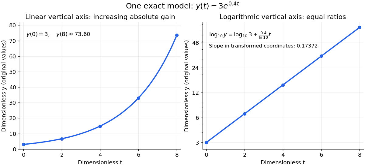
The same exponential growth model bends on a linear scale and is straight on a semi-log plot with a logarithmic vertical axis
. Original exact mathematical model , not measurements. Both panels show identical values at the same . Right-hand tick labels retain the original values, with equal gaps for each doubling. The stated slope is for , not the original derivative . Details.One practical use is checking a proposed exponential distribution for failure times. For rate and , its cumulative distribution function is , so the reciprocal survival function satisfies . Estimated probabilities can therefore be placed on a logarithmic vertical axis and compared with a straight line. Agreement supports compatibility with the chosen statistical model; a roughly straight finite sample does not establish a unique physical mechanism.[ref]
8.2.2.1. Probability plotting. NIST and SEMATECH e-Handbook of Statistical Methods, §8.2.2.1 Probability plotting: Exponential Model, logarithmic vertical-axis transformation and interpretation of approximate straightness
Pinned article: Introduction to the OurBigBook Project
Welcome to the OurBigBook Project! Our goal is to create the perfect publishing platform for STEM subjects, and get university-level students to write the best free STEM tutorials ever.
Everyone is welcome to create an account and play with the site: ourbigbook.com/go/register. We belive that students themselves can write amazing tutorials, but teachers are welcome too. You can write about anything you want, it doesn't have to be STEM or even educational. Silly test content is very welcome and you won't be penalized in any way. Just keep it legal!
Intro to OurBigBook
. Source. We have two killer features:
- topics: topics group articles by different users with the same title, e.g. here is the topic for the "Fundamental Theorem of Calculus" ourbigbook.com/go/topic/fundamental-theorem-of-calculusArticles of different users are sorted by upvote within each article page. This feature is a bit like:
- a Wikipedia where each user can have their own version of each article
- a Q&A website like Stack Overflow, where multiple people can give their views on a given topic, and the best ones are sorted by upvote. Except you don't need to wait for someone to ask first, and any topic goes, no matter how narrow or broad
This feature makes it possible for readers to find better explanations of any topic created by other writers. And it allows writers to create an explanation in a place that readers might actually find it.
Figure 1. Screenshot of the "Derivative" topic page. View it live at: ourbigbook.com/go/topic/derivativeVideo 2. OurBigBook Web topics demo. Source. - local editing: you can store all your personal knowledge base content locally in a plaintext markup format that can be edited locally and published either:This way you can be sure that even if OurBigBook.com were to go down one day (which we have no plans to do as it is quite cheap to host!), your content will still be perfectly readable as a static site.
- to OurBigBook.com to get awesome multi-user features like topics and likes
- as HTML files to a static website, which you can host yourself for free on many external providers like GitHub Pages, and remain in full control

Figure 2. You can publish local OurBigBook lightweight markup files to either OurBigBook.com or as a static website.
Figure 3. Visual Studio Code extension installation.
Figure 5. . You can also edit articles on the Web editor without installing anything locally. Video 3. Edit locally and publish demo. Source. This shows editing OurBigBook Markup and publishing it using the Visual Studio Code extension. 
- Infinitely deep tables of contents:




All our software is open source and hosted at: github.com/ourbigbook/ourbigbook
Further documentation can be found at: docs.ourbigbook.com
Feel free to reach our to us for any help or suggestions: docs.ourbigbook.com/#contact