For the wave equation ${\psi }_{tt}=c^2{\psi }_{xx}$ on $0<x<L$, impose homogeneous Neumann boundary conditions ${\psi }_x(0,t)={\psi }_x(L,t)=0$, where $c,L>0$. Separation of variables gives $X^{\prime \prime }+\lambda X=0$ and $T^{\prime \prime }+c^2\lambda T=0$. Integration by parts gives ${\int }_0^L(X^{\prime }{)}^{2}dx=\lambda {\int }_0^L{X}^{2}dx$, so every nontrivial spatial eigenfunction has $\lambda \ge 0$.

For $\lambda =0$, $X$ is constant and $T=A_0+B_{0}t$. For $\lambda >0$, the boundary conditions select ${\lambda }_n=(n\pi /L{)}^2$ and $X_n=\cos (n\pi x/L)$. The superposition principle gives the displayed expansion when the initial data have sufficient regularity. The constant zero mode must be retained: homogeneous Neumann boundary conditions do not force the spatial average of the displacement to vanish.

With zero initial velocity, all $B_n$ vanish, including $B_0$. Initial displacement $a+b\cos (n\pi x/L)$ then evolves as $a+b\cos (cn\pi t/L)\cos (n\pi x/L)$, a standing wave above a constant offset.

A strip of membrane with fixed edges $y=0,b$ supports transverse normal modes proportional to $\sin (n\pi y/b)$, $n\ge 1$. Separation of the two-dimensional wave equation gives the displayed dispersion relation. Confinement produces longitudinal wave dispersion even when the membrane's underlying wave speed $v$ is independent of frequency.

For $y_{tt}-y_{xx}=F(t)\delta (x-x_0)$ with zero endpoint displacement, a Fourier sine series gives $q_n^{\prime \prime }+k_n^2{q}_n=2F(t)\sin (k_n{x}_0)/L$. With the $e^{-i\omega t}$ Fourier transform convention, the causal inverse of this oscillator uses the displayed denominator. Its inverse transform is $H(t)\sin (k_{n}t)/k_n$, giving $q_n(t)=2\sin (k_n{x}_0)/(L{k}_n){\int }_{-\infty }^{t}F(s)\sin [k_n(t-s)]ds$ when the past integral exists. The plain denominator $k_n^2-{\omega }^2$ requires a pole prescription: its Cauchy principal value gives the time-symmetric kernel $\sin (k_n|t|)/(2k_n)$ instead. Homogeneous sine and cosine modes are additional freedom unless temporal data or causality are specified.

For real constants $\gamma ,c$, the substitution $v=e^{\gamma t}u$ turns the displayed equation into the wave equation $v_{tt}=c^2{v}_{xx}$. If $u(x,0)=f(x)$ and $u_t(x,0)=g(x)$, then $v(x,0)=f(x)$ and $v_t(x,0)=g(x)+\gamma f(x)$. For $v_0=|c|>0$, D'Alembert's formula consequently givesThe extra $\gamma f$ term is necessary even when the original initial velocity is zero. For $c=0$, take the limit to obtain $u=e^{-\gamma t}[f+t(g+\gamma f)]$. The formula gives classical solutions for suitably smooth data and weak solutions for less regular data. Positive $\gamma$ damps the transformed wave, whereas negative $\gamma$ amplifies it.

A wave equation with a linear damping term and positive wave speed $c$ separates into spatial normal modes and damped harmonic oscillators. For a spatial eigenvalue $k^2$, the time factor obeys $T^{\prime \prime }+\alpha T^{\prime }+c^2{k}^{2}T=0$. Its characteristic roots are $-\alpha /2\pm \sqrt{{\alpha }^2/4-c^2{k}^2}$. Thus underdamping requires $|\alpha |<2c|k|$, critical damping gives a repeated root and the second solution $t{e}^{-\alpha t/2}$, and overdamping gives two real exponential rates. Negative $\alpha$ amplifies rather than damps the motion.

A fixed circular elastic membrane of radius $a$ has radial normal modes satisfying the displayed Sturm-Liouville problem, with weight $r$, $R(a)=0$ and regularity at the origin. The regular solutions are Bessel functions of the first kind $J_0(\sqrt{\lambda }r)$. Integration by parts gives the positive Rayleigh quotient $\lambda ={\int }_0^{a}r|R^{\prime }{|}^{2}dr/{\int }_0^{a}r|R{|}^{2}dr$. Distinct modes are orthogonal in the weighted inner product ${\int }_0^{a}r\overline{R}Sdr$.

A vortex ring is a vortex tube bent into a closed loop, often approximately a circle. Its vorticity runs around the loop, while the induced velocity field passes through the centre and returns outside. For a thin ring of radius $r$ and circulation $\Gamma$, the Biot-Savart law for incompressible vorticity gives an axial velocity $u_z(z)=\Gamma r^2/[2(r^2+z^2{)}^{3/2}]$, measured relative to the ring centre, with its sign set by the circulation orientation. A vortex ring is not a loop of fluid whose velocity everywhere merely follows the circular vortex line.

A vortex filament is the ideal thin-core limit of a vortex tube, concentrating a finite circulation on a curve. In an unbounded incompressible fluid with velocity tending to zero at infinity, its induced velocity field follows the vorticity version of the Biot-Savart law. The ideal field is singular on the filament; finite-core models are needed there. A closed circular filament is a thin vortex ring.

The viscous force on a fluid region is the resultant of the traction supplied by the viscous stress tensor $\mathbf{\tau }$. With $\mathbf{n}$ the outward unit normal of the region, its surface contribution is the displayed surface integral. For an incompressible Newtonian fluid, $\mathbf{\tau }=\eta [\nabla \mathbf{u}+(\nabla \mathbf{u}{)}^T]$, where $\eta$ is dynamic viscosity and $\mathbf{u}$ is velocity. A force scale is $\eta UL$ for a body of size $L$ moving at speed $U$, while the inertial force scale is $\rho U^2{L}^2$; their ratio is the Reynolds number. Total hydrodynamic drag on a body includes both viscous traction and the pressure traction induced by the flow. For example, the full Stokes drag law gives $6\pi \eta RU$ for a no-slip sphere, rather than just the viscous-traction part alone.

François Viète studied the connection between positive roots of a polynomial and the coefficients of the powers of the unknown. His 1591 presentation of algebraic notation used letters for both known and unknown quantities, with consonants for known quantities and vowels for unknown quantities. That move makes it possible to express a relation for whole families of polynomials, rather than only a numerical instance. His historical setting concerned positive roots and expressions satisfying dimensional homogeneity; the modern splitting field formulation above is a broader statement.^[ref]

For the quadratic polynomial $p(x)=2x^2-6x+5$, the discriminant is $(-6{)}^2-4(2)(5)=-4$, so its roots of a polynomial are the complex conjugatesTheir sum is $3=-(-6)/2$, and their product is $(9+1)/4=5/2$, matching the constant coefficient divided by the leading coefficient. More revealingly, $r_{+}{r}_{-}=r_{+}\overline{r_{+}}=|r_{+}{|}^2$: the product is the square of a complex modulus. Coefficients in the real numbers therefore need not imply polynomial roots in the real numbers.

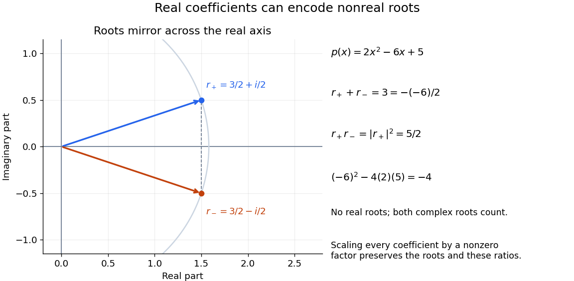
For any polynomial with coefficients in the real numbers, $p(\overline{z})=\overline{p(z)}$. Thus a nonreal root of a polynomial brings its complex conjugate along with the same multiplicity of a root. This follows by applying complex conjugation to the polynomial expression and its factors. It explains why sums of complex conjugate terms can produce coefficients in the real numbers.

For the polynomial $(x-2{)}^2(x+1)=x^3-3x^2+4$, the root list is $2,2,-1$, not $2,-1$. Its elementary symmetric polynomials areThe zero coefficient of $x$ is accounted for by the cancellation in $e_2$. Omitting one occurrence of the double root of a polynomial loses both the polynomial degree and the correct coefficients. Multiplicity of a root is part of the root data.

Take the stipulated polynomial roots $-2,1,5$. Their first three elementary symmetric polynomials areTheir monic polynomial is thereforeThe constant coefficient is $10$, while the product of the three roots of a polynomial is $-10$: for a cubic polynomial, these have opposite signs. Expanding the factors directly verifies the same polynomial identity.

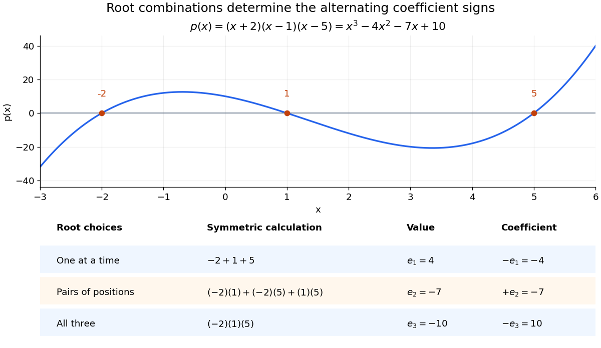
For the nonmonic polynomial $-3x^3+12x^2+21x-30$, the same ratios give sum $-12/(-3)=4$, pairwise-product sum $21/(-3)=-7$, and product $-(-30)/(-3)=-10$. It is $-3$ times the monic polynomial above, so its roots of a polynomial are the same. Checking only the sum and product would leave the middle elementary symmetric polynomial unchecked; all three are needed to recover a monic polynomial of polynomial degree three.

In 1851 Hippolyte Fizeau detected a change in light propagation through moving water using interference fringes. Sunlight entered a telescope through a partially reflecting mirror; two slits selected beams passing through parallel glass tubes, each $1.487\mathrm{m}$ long with $5.3\mathrm{mm}$ internal diameter. A second telescope and focal mirror exchanged the tubes on return, and the beams recombined at a graduated eyepiece. Compressed air drove water between reservoirs, producing opposite flows; reversing both flows reversed the interference fringe displacement. The double transit suppressed static differences in temperature and pressure; filling only one tube with water tested this compensation. Separate supports reduced mechanical disturbance. Hippolyte Fizeau estimated flow speed from volumetric flow rate divided by tube cross section.^[ref]

The Fizeau experiment turns a tiny change in phase velocity into a visible fraction of an interference fringe. The Fizeau experiment path-length convention below explains why both tube passages contribute with the same sign for one beam and the opposite sign for the other. This makes the apparatus sensitive to the part of the phase difference that reverses with the flow, while rejecting disturbances shared by both beams.

A neutral vector meson of spin-parity $1^{-}$, predominantly $s\bar{s}$ in the ideal quark-flavour description. A pseudoscalar decaying to this meson and a pion requires relative orbital angular momentum one if total angular momentum is zero.

For pairwise-additive nonretarded molecular attraction and equal solid number densities $n$, let $A_H={\pi }^{2}B{n}^2$ and let $L>R$ be the distance from a sphere centre to a planar half-space. Integrating the atom–half-space potential energy givesFor $L\gg R$, expansion gives the displayed expression. Equivalently expand $(L+z{)}^{-3}$ over the sphere: its odd moments vanish and $⟨z^2⟩=R^2/5$. This yields the first relative correction $6R^2/(5L^2)$. In the opposite near-contact limit, the gap $h=L-R\ll R$ gives $U\simeq -A_{H}R/(6h)$ and the sphere-plane dispersion force magnitude $A_{H}R/(6h^2)$. The two limits use different distances and must not be confused.

NASA's Wind Tunnel Experiment Details, slide 27, describes a practical manometer measurement: partially fill a Tygon tube with water and connect its two ends to total pressure and static pressure ports in a wind tunnel. The total pressure connection pushes its liquid meniscus downward; the vertical length difference supplies the pressure difference. The slide predicts increasing separation as the tunnel speed increases. It supplies an apparatus and method, rather than a table of observed readings.^[ref]

A control for this practical is to expose both connections to the same atmospheric pressure before the run: settled liquid meniscus heights should agree in a symmetric column. Read each liquid meniscus at eye level, reconnect sealed tubing to the identified ports, and wait for settling. Recheck the equal-pressure zero afterwards; reverse connections to check the sign. These checks establish neither mass density nor ruler accuracy.^[ref]

The inference is a differential pressure from hydrostatic pressure, with stagnation pressure on one side and static pressure on the other in NASA's practical. Converting that difference to a flow speed additionally needs the hypotheses discussed under dynamic pressure and Pitot-static tube. A changing pressure can leave the column oscillating; leaks, blocked pressure tappings or trapped liquid in a gas connection can alter or delay the readout. The column should be read after settling, and temperature should be recorded when choosing the measuring liquid's mass density.

Two corrections clarify the limits. If both gas ports are at the same height and carry the same gas of constant mass density ${\rho }_g$, keeping its hydrostatic pressure gives $p_L-p_R=(\rho -{\rho }_g)g\Delta h$. Different port heights require their separate gas column heights. Also, a curved liquid meniscus can sustain a capillary pressure jump through surface tension. Write $J_L,J_R$ for liquid pressure minus gas pressure at the two surfaces. Neglecting gas weight, the balance becomes $p_L-p_R=\rho g\Delta h+J_R-J_L$. Identical meniscus shapes in matching clean bores cancel those jumps; unequal bores or different wetting conditions need not. Thus the useful simplicity of $\rho g\Delta h$ rests on identifiable physical conditions.

The ideal measurement calibration is a straight line through the equal-pressure zero. For the stipulated water mass density and gravitational acceleration above, its slope is $9.81\mathrm{Pa}$ per vertical millimetre. A lower liquid mass density gives a larger length change for the same pressure, improving the height-reading contribution to measurement resolution but requiring more vertical space for a given pressure range. The pressure scale depends on the actual mass density, which depends on temperature; $1000\mathrm{kg}{\mathrm{m}}^{-3}$ here is a chosen model value, not an exact property of all water samples.

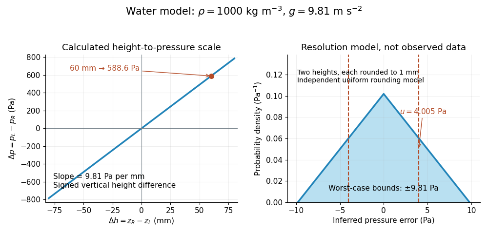
Suppose each liquid meniscus height is rounded to the nearest scale division $q=1\mathrm{mm}$. Each height measurement error lies within $q/2$, so the error in their difference lies within $q$. The resulting pressure error is bounded by $\rho gq=9.81\mathrm{Pa}$. To quantify a standard uncertainty, make the additional model assumption that the two rounding errors are independent random variables, each having a continuous uniform distribution on $[-q/2,q/2]$. Each then has variance $q^2/12$; adding the two variances givesHere $u$ denotes standard uncertainty. The $9.81\mathrm{Pa}$ worst-case bound and $4.0049\mathrm{Pa}$ standard uncertainty answer different questions. At $588.6\mathrm{Pa}$ they are respectively $1.67\%$ and $0.680\%$ of the reading. Shared reading bias or a different reading method can violate the assumed independence.

If the mass density, gravitational acceleration and height difference also have small independent standard uncertainties, a first-order estimate follows from the partial derivatives of $\Delta p=\rho g\Delta h$:This displays why a finer scale does not remove uncertainty in mass density or gravitational acceleration. A pressure transducer compared against the column needs its own differential-pressure calibration to establish an electrical response.

The High-Z Supernova Search Team analysis fitted multicolour light curves and interstellar extinction, and compared a second decline-rate method. Similar local and distant spectroscopy supported, but did not establish, population stability. Nearly colourless attenuation remained a qualified alternative.^[ref]

The Supernova Cosmology Project compared low- and high-redshift colours, removed red outliers in its primary fit, and tested Malmquist bias with artificial-source recovery.^[ref]

The inference can be organized as a chain of independently testable failure modes. A magnitude zero point offset between nearby and distant observations imitates a distance modulus offset; a common offset instead changes the intercept. An erroneous photometric passband response changes a K correction in a redshift-dependent way because different emitted wavelengths cross the detector band. Residual host-galaxy light changes the recovered radiative flux. Color excess constrains wavelength-dependent interstellar extinction only after intrinsic colour is modeled; grey attenuation is not bounded by colour alone. Changes in stellar population or metallicity could shift standardized absolute magnitude without large changes in the chosen shape parameter. These are logical degeneracies, so increasing the sample size alone cannot remove them.

A useful control strategy therefore compares subsets with different host environments, fits consistent rest-frame photometric passbands, and checks artificial-source recovery through the same image processing and selection. A Malmquist bias tends to select brighter detectable sources, but the relative bias between the nearby and distant samples is what matters. Peculiar velocity mainly perturbs the nearby redshift anchor; weak gravitational lensing changes individual brightnesses and the selection distribution. Neither can be replaced by an arbitrary extra scatter term when its mean or selection dependence is uncertain.