For a linear system ${\sum }_j{a}_{ij}{x}_j=b_i$, the coefficient matrix $A$ contains the coefficients of the unknowns, with one row per equation and one column per unknown. The system becomes $A\mathbf{x}=\mathbf{b}$. The augmented matrix $[A\mid \mathbf{b}]$ additionally includes the right-hand-side column; that column is not part of $A$.

The $S=1$ Heisenberg antiferromagnet chain realizes the Haldane phase: a gapped symmetry-protected topological phase with effective spin one-half degrees of freedom at open ends. Time-reversal symmetry is one possible protecting symmetry. Integer spin alone does not imply the same protected class: odd- and even-integer chains differ. The broader gap distinction is the Haldane conjecture.^[ref]

For an axially symmetric rigid body with $I_1=I_2=I_{\perp }$ and $I_3=I_{\parallel }$, no external torque means that angular momentum $\mathbf{L}$ is fixed in an inertial frame. The axial angular velocity ${\omega }_3$ is constant by Euler equations for a torque-free rigid body, and the symmetry axis obeysIts angle to $\mathbf{L}$ is constant and it precesses in space at $L/I_{\perp }$. The transverse angular-velocity components instead rotate in body coordinates at signed rate $(I_{\parallel }-I_{\perp }){\omega }_3/I_{\perp }$. These are different frame descriptions and must not be substituted for one another.

Let $v$ be a real unit vector in $d$-dimensional Euclidean space. Then $P=v{v}^{\mathsf{T}}$ is a rank-one orthogonal projection: $Pv=v$, while $Pw=0$ for $w$ orthogonal to $v$. Consequently the symmetric matrix $A=\alpha I+\beta P$ has eigenvalue $\alpha +\beta$ on the line spanned by $v$ and eigenvalue $\alpha$ on its orthogonal complement. Any orthonormal basis of that complement completes $v$ to an orthonormal eigenbasis. ThusThe trace and determinant formulas remain valid when one of these eigenvalues is zero. When $\beta =0$, all nonzero vectors have the same eigenvalue, and the chosen splitting is optional.

A detergent is a substance or formulation that assists cleaning, commonly through surfactants with water-compatible and oil-compatible molecular regions. These molecules collect at interfaces and can form micelles that help disperse oily material in water. Agitation, concentration and the composition of both the soil and washing solution affect the process.

A simple comparison is to shake an oil-water mixture with and without a suitable detergent and observe how readily droplets disperse and how long they persist. Lowering surface tension can improve wetting, while adsorption and aggregation change how oily material is carried away. Stable dispersion and removal are different steps: the surrounding fluid must still transport the dispersed material.

Detergents can also disrupt a lipid bilayer. In a protease protection assay, removing that membrane barrier tests whether it caused the apparent protection of an enclosed protein.

Soap consists of sodium or potassium salts of long-chain fatty acids. Its hydrophilic carboxylate head and hydrophobic hydrocarbon tail make it an amphiphile; saponification of triglycerides produces these salts.

An anionic surfactant with a twelve-carbon hydrocarbon tail and a negatively charged sulfate head group, accompanied by a sodium counterion. This separation of hydrophobic and hydrophilic regions makes it an amphiphile. It forms aqueous micelles under suitable concentration and temperature conditions and is used in sodium dodecyl sulfate polyacrylamide gel electrophoresis.

A cationic surfactant with a sixteen-carbon hydrocarbon tail and a positively charged trimethylammonium head group, accompanied by a ${\mathrm{Br}}^{-}$ counterion. It is an amphiphile that can form aqueous micelles. Its head-group charge has the opposite sign to that of sodium dodecyl sulfate.

A toroid is a ring-shaped surface of revolution obtained by rotating a closed planar profile about an axis in its plane that stays outside the profile. A circular profile gives a torus; a rectangular profile gives a ring with rectangular cross-section. The enclosed solid supplies the core geometry in a toroidal winding, while the mathematical surface is its boundary. The distinction matters when computing a surface area versus a volume.

For surface-fed growth of an accreting sphere with $\mu =\dot{r}>0$, stationary incoming material, and quadratic drag $F_D=C_D{\rho }_a\pi r^2{v}^2/2$, the variable-mass system obeys $\dot{v}+3\mu v/r=g-3C_D{\rho }_a{v}^2/(8\rho r)$. For constant positive parameters, $r\sim \mu t$ and the late balance gives the displayed speed. The omitted acceleration and accretion terms are both $O(t^{-1/2})$, consistent with the balance. Thus this growing sphere has unbounded speed with vanishing acceleration, rather than a finite terminal velocity. This model has a different growth law from the existing accreting raindrop with quadratic drag, whose growth rate is proportional to speed.

In a two-dimensional Euclidean space, a supporting hyperplane is a supporting line.

Sagittarius A* is the compact radio source at the centre of the Milky Way. Nearby infrared stars allow its central mass concentration to be studied through their orbits.^[ref]

In the two-fluid model of superfluidity, the superfluid fraction is ${\rho }_s/\rho$, where ${\rho }_s$ is the superfluid mass density and $\rho$ the total mass density. For a one-component fluid of particles of the same mass this also equals $n_s/n$, using the superfluid number density $n_s$ and total number density $n$. It measures the superfluid response and is distinct from the condensate fraction, which measures occupation of a single-particle state. Interactions can make the two fractions very different.

The Landau criterion asks whether creating an excitation can lower a moving superfluid's energy. For a weakly coupled, heavy obstacle moving through a uniform liquid initially at zero temperature, let $ϵ(p)>0$ be the excitation energy in the fluid rest frame, with momentum magnitude $p$. Transferring momentum $\mathbf{p}$ from an obstacle moving at velocity $\mathbf{v}$ supplies, to leading order in its negligible recoil, energy $\mathbf{v}\cdot \mathbf{p}$. Emission requiresFor an isotropic dispersion relation, the easiest direction is parallel to $\mathbf{v}$, giving the necessary kinematic conditionAn infimum includes cases in which the limiting slope occurs only as $p\to 0$. A finite-mass obstacle of mass $M$ instead loses $\mathbf{v}\cdot \mathbf{p}-p^2/(2M)$, so the corresponding emission inequality includes the extra positive recoil term $p^2/(2M)$ on the left. This is an energy and momentum balance, not a calculation of an emission rate.

The Landau criterion excludes spontaneous emission into the specified spectrum below its threshold. Above it, kinematic permission alone does not guarantee strong coupling or rapid decay. It is not a universal observed flow threshold: walls, channel geometry and quantum vortex nucleation can enable other decay routes, and finite temperature permits scattering from existing excitations. Using only bulk phonons and rotons leaves those processes outside the model.

Landau's 1941 energy and momentum argument used a roton approximation different from the finite-momentum minimum illustrated below.^[ref]

Landau received his Nobel Prize in Physics in 1962 while hospitalized in Moscow after a car accident.^[ref]

For a deliberately simple Bose-Einstein condensation comparison, stipulate an ideal free-particle excitation law $ϵ=p^2/(2m)$. Then $ϵ/p=p/(2m)$ has infimum zero. Macroscopic one-particle occupation therefore supplies no positive emission threshold by this argument alone. By contrast a linear phonon law $ϵ=cp$ yields $v_L=c$. The dispersion relation and the collective response contain information that the occupation criterion alone does not supply; Bose-Einstein condensation and thermodynamic superfluidity must be tested separately.

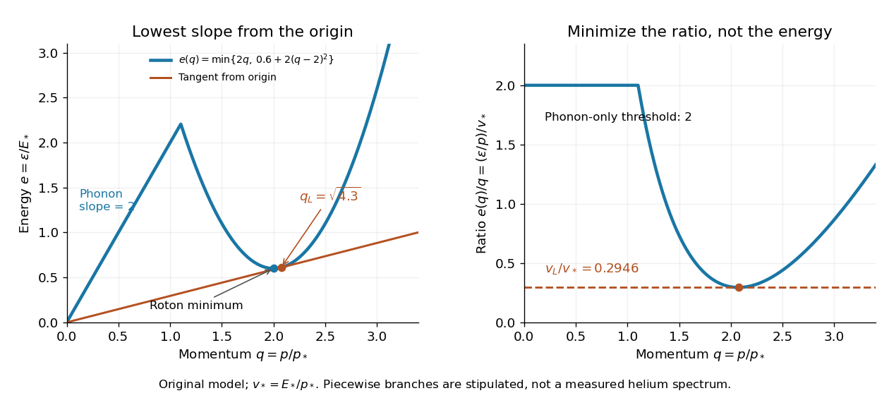
To check the picture algebraically, on the stipulated roton branch,Thus tangency occurs at $q_L=\sqrt{4.3}$, slightly above the roton energy minimum. At an energy minimum $e^{\prime }=0$, but a tangent through the origin needs $e^{\prime }=e/q>0$. Minimizing energy and minimizing the energy-to-momentum ratio are different operations. This geometric construction makes the criterion useful even when the full dispersion relation is supplied numerically rather than by a simple formula.

A spatial image after a chosen dark interval is a different readout from continuously recording arrivals at a fixed probe. Here is an original idealised fluorescence imaging model: release a dilute cloud, let it move freely, then apply a short uniform probe pulse. Neglect collisions, residual forces, attenuation and motion during the pulse. Use each image's cloud centre to remove mean drift. Uniform gravity shifts that centre without changing the centred variance.

For each atom let $x(t)=x_0+v_{0}t$ along a horizontal imaging axis. Expanding the square about the expected values gives exactlyNo Gaussian distribution is needed for this variance identity. A jointly Gaussian distribution of initial positions and velocities does make the later density Gaussian. For a separable three-dimensional cloud viewed along $z$, integration along the viewing direction gives the column densityHere $N$ is atom number. Integrating this image along $y$ leaves a one-dimensional Gaussian distribution with standard deviation ${\sigma }_x(t)$. This is a projected density measurement, not a three-dimensional radius or a direct velocity histogram. Under the uniform, optically thin probe assumptions, expected fluorescence is proportional to this column density. A known, independent point spread function with finite variance adds its own variance to the measured width; probe duration and intensity gradients need separate treatment.

For a Maxwell-Boltzmann distribution, $T_x=m{\sigma }_v^2/k_B$, where $m$ is atomic mass and $k_B$ the Boltzmann constant. For a nonthermal distribution this defines a directional second-moment temperature, which need not describe every feature of the distribution. A covariance between position and velocity can initially narrow the cloud even though ${\sigma }_v^2$ is positive. The physical covariance matrix requires $C_{xv}^2\le {\sigma }_{x0}^2{\sigma }_v^2$.

Choose ${\sigma }_{x0}=0.60\mathrm{mm}$, ${\sigma }_v=0.060\mathrm{m}{\mathrm{s}}^{-1}$ and $C_{xv}=-0.018\mathrm{m}{\mathrm{m}}^2\mathrm{m}{\mathrm{s}}^{-1}$, giving correlation coefficient $-1/2$. With $t$ in milliseconds, the numerical variance in square millimetres is $0.36-0.036t+0.0036t^2$. Its minimum occurs at $5\mathrm{ms}$, with standard deviation $\sqrt{0.27}\mathrm{mm}$. These chosen values satisfy the covariance matrix constraint; early contraction is compatible with free motion.

Generate thirteen synthetic variance observations at equally spaced times from $0$ to $30\mathrm{ms}$, adding independent Gaussian noise of standard deviation $0.012\mathrm{m}{\mathrm{m}}^2$. Linear least squares fits all three coefficients in $a+bt+c{t}^2$. The example yields $a\simeq 0.37026\mathrm{m}{\mathrm{m}}^2$, $b\simeq -0.036413\mathrm{m}{\mathrm{m}}^2\mathrm{m}{\mathrm{s}}^{-1}$ and $c\simeq 0.0035820\mathrm{m}{\mathrm{m}}^2\mathrm{m}{\mathrm{s}}^{-2}$. With the chosen approximate sodium mass $m=3.82\times 10^{-26}\mathrm{kg}$, the true $T_x$ is $9.96\mu \mathrm{K}$ and the fitted value is $9.91\mu \mathrm{K}$. This is a fit to generated width data, not historical observations.

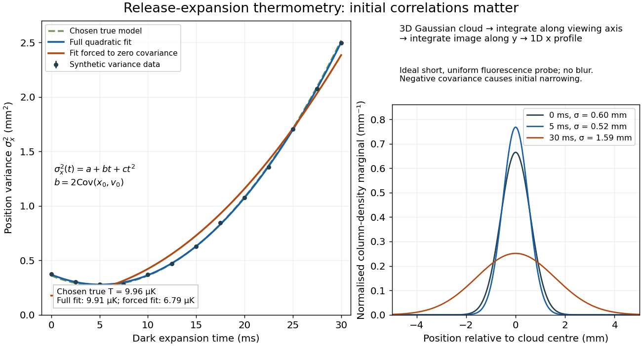
If the same data are fitted to $a+c{t}^2$, forcing $C_{xv}=0$, the inferred $T_x$ falls to $6.79\mu \mathrm{K}$. The omitted term is partly absorbed into both fitted coefficients. In noiseless linear least squares with a free intercept, its precise effect on the quadratic coefficient iswhere the subscript denotes equal-weight moments over the chosen observation times, using one consistent unit system. Since the ratio is positive for distinct nonnegative times, negative $C_{xv}$ biases this estimate downwards. An incorrect release-time origin can also generate a linear term, so fitting it does not by itself identify a physical initial covariance. Timing calibration, spatial resolution, residual magnetic fields and probe-induced recoil energy remain separate controls. Neither a cold-looking image nor a single long expansion time identifies all three coefficients.

The 1988 experiment loaded sodium optical molasses from a slowed atomic beam. After stopping loading, a shutter extinguished the six cooling beams. Released atoms crossed a lower probe; a photomultiplier recorded fluorescence versus arrival time. Calculations integrated the measured initial cloud distribution and an assumed three-dimensional Maxwell-Boltzmann distribution, including gravity and detection geometry. The minimum was $43\pm 20\mu \mathrm{K}$, versus the $240\mu \mathrm{K}$ Doppler cooling limit.^[ref]

Probe separation, probe intensity, cloud density and shutter timing were varied. Fountain-height, horizontal-spreading and release/recapture measurements also gave below-limit results. Geometry remained an uncertainty; agreement among complementary thermometers made a detector artifact less plausible. These measured released atoms, rather than an in-situ velocity distribution.^[ref]

Steven Chu's account connects the explanation to optical pumping, Stark effect shifts and spatially changing electromagnetic polarization; Claude Cohen-Tannoudji's lecture separates this mechanism from subrecoil schemes. Their lectures and William D. Phillips's describe complementary experimental and theoretical routes.^[ref][ref]

For the radial Laplace operator $L=-r^{-2}(r^2{u}^{\prime }{)}^{\prime }$ on $0<r<R$, require a finite value at the origin and $u(R)=0$. The map $u\mapsto v=ru$ preserves the norm from $L^2((0,R),r^{2}dr)$ to $L^2(0,R)$ and sends $L$ to $-d^2/d{r}^2$. The regular endpoint condition becomes $v(0)=0$. The self-adjoint realization therefore corresponds to the ordinary Dirichlet boundary conditions for the one-dimensional second derivative. Its eigenvalues and eigenfunctions are displayed above, with $u_n(0)=n\pi /R$ understood by a limit. Their squared weighted norm is $R/2$. Completeness and orthogonality follow from the Fourier sine series on $(0,R)$.

For $\ell >0$ and $k>0$, the Sturm-Liouville problem with one Dirichlet boundary condition and one Robin boundary condition has positive eigenvalues. Indeed, integration by parts givesfor every nonzero eigenfunction. Let $z=\ell \sqrt{\lambda }$ and $\kappa =k\ell$. The eigenfunctions are proportional to $\sin (zx/\ell )$, withFor each $n\ge 1$, there is exactly one root $z_n$ in $((n-1/2)\pi ,n\pi )$: on that interval $\tan z+z/\kappa$ increases strictly from $-\infty$ to a positive value. There are no other positive roots. The apparent root $z=0$ gives only the zero sine function and is not an eigenvalue.

For fixed $k,\ell$, write $z_n=(n-1/2)\pi +{\epsilon }_n$. The root equation becomes $\kappa \cot {\epsilon }_n=(n-1/2)\pi +{\epsilon }_n$, henceAn optional unit normalization uses ${\int }_0^{\ell }{\sin }^2(\sqrt{{\lambda }_n}x)dx=\ell /2+k/[2(k^2+{\lambda }_n)]$. The positive sign of the Robin boundary term matters: reversing it can introduce nonpositive modes, as in nonpositive modes in a Dirichlet-Robin interval expansion.

Suppose $p(x)=c(x-a)+O((x-a{)}^2)$ with $c>0$, and the other coefficients in $(p{y}^{\prime }{)}^{\prime }+(\lambda w-q)y=0$ extend continuously to $a$, with $w(a)>0$. A bounded eigenfunction has $(p{y}^{\prime }{)}^{\prime }=O(1)$, hence $p{y}^{\prime }=C+O(x-a)$. A nonzero $C$ would give $y^{\prime }\sim C/[c(x-a)]$ and an unbounded logarithmic singularity. Thus $C=0$, and the regular branch has bounded first derivative. The second local branch carries a logarithm. The title condition excludes that branch.

For two regular eigenfunctions, $p(\overline{u}{v}^{\prime }-\overline{u^{\prime }}v)\to 0$. This removes the singular-end contribution to the Lagrange identity for a Sturm-Liouville operator. Together with a separated self-adjoint condition at the other endpoint, it selects the regular self-adjoint differential operator realization. The precise operator domain uses the maximal differential-operator domain and the no-log endpoint condition; boundedness of classical eigenfunctions is its convenient local expression, not a replacement for specifying an operator domain.