Topics (384k) Articles (398k) Users (410) Discussions (242) Comments (383) Files (13k) New article
Keep the original all-to-one orientation of the Bellman inequalities: concerns routes from to a fixed sink , and belongs to the original directed edge . Initialize and for . The synchronous dynamic programming recurrence isIt prepends the first edge of a route instead of appending the last: is the minimum cost of a directed walk from to using at most edges. In particular, improving can improve labels on incoming directed edges . The same original directed edge therefore updates its tail in this convention, whereas single-source edge relaxation updates its head.
If no negative-cost directed cycle can reach , rounds suffice for every distance to , and automatically. This hypothesis concerns directed paths from the cycle to the sink, not paths from the sink to the cycle. In the base example with its original arrows and sink , the distances in order are . Once of weight is added, instead have distance to , while keeps distance and keeps .
More generally, precisely when can reach a negative-cost directed cycle that can reach . Thus the affected vertices are the ancestors of such a directed cycle. A negative-cost directed cycle unable to reach is irrelevant. Reversing all arrows makes a single source, turns these ancestors into descendants, and makes the detection and forward graph search above directly applicable. The right panel of the figure uses that reversal with sink ; its distances to equal the left panel's distances from .
Do not force the root to remain zero outside the hypothesis. Consider the two directed edges of cost and of cost , with sink . The recurrence gives and : the latter records one lap of a negative-cost directed cycle through . Repetition makes both unrestricted distances . Clamping at zero and omitting its update would instead leave the stationary labels , concealing that behaviour. Initialization specifies the cost of the empty directed walk; it does not forbid cheaper nonempty returns to the root. Cycle detection must test every relevant directed edge, including those whose relaxation updates the root.
A negative-cost directed cycle matters to a particular destination precisely when it is reachable from and can itself reach .[ref]
Lecture 17: Shortest Paths III: Bellman-Ford. 6.006 Introduction to Algorithms, Fall 2011 by Massachusetts Institute of Technology, 6.006 course staff; MIT 6.006, Lecture 17, p. 1: cycle between source and destination; p. 4: reachable-cycle corollary
Repeating it times adds times its negative total cost to a route. Thus the infimum of directed walk costs is , rather than the cost of a finite shortest directed walk. The distinction is about reachability, not simply the presence of a negative edge or a negative-cost directed cycle anywhere in the graph.Add of weight to the worked example. Now has total weight . Add also an isolated vertex with a self-loop of weight . From , the distances of are , because all four are reachable from the first negative-cost directed cycle. The source retains distance : no directed edge leads back to . The unreachable retains distance , despite its negative-cost self-loop.
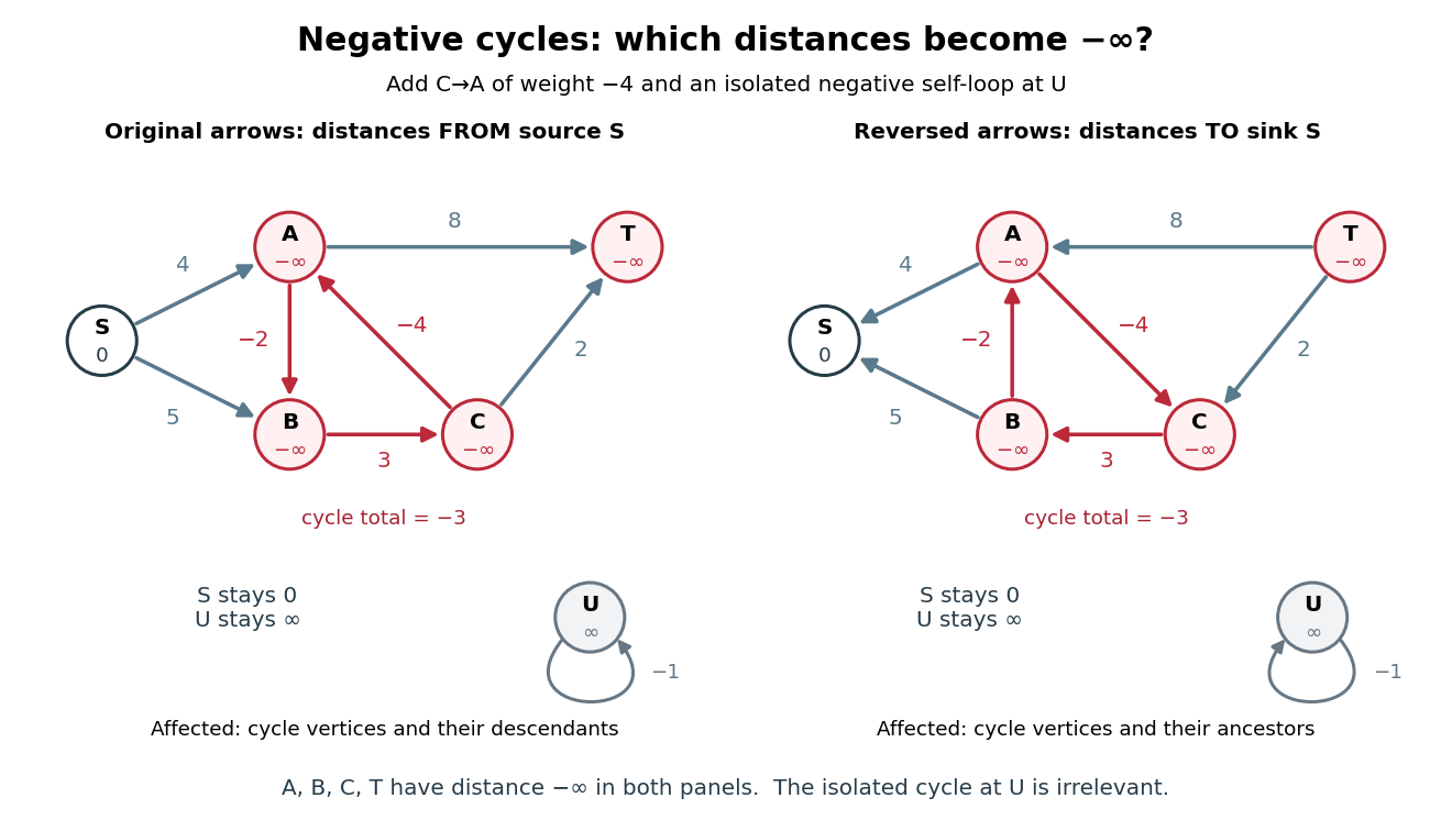
Relevant negative-cost directed cycles: descendants from a source become ancestors when every directed edge is reversed
. Details. For example, extra laps before proceeding to give costs . This construction also shows why requiring a directed path with no repeated vertices would change the problem: only directed walks permit arbitrarily many laps. Merely finding one reachable negative-cost directed cycle does not justify setting every reachable label to ; in the figure is a counterexample.
To detect and classify, perform full passes without clamping any label, then test all directed edges against a fixed copy of the resulting labels. Collect heads of edges satisfying and . An empty collection certifies that no negative-cost directed cycle is reachable from . Otherwise run graph search forwards from all collected vertices: precisely the reached vertices have distance . A vertex unreachable from still has distance ; each remaining vertex has its finite shortest distance.
Why is this classification exact? Every unaffected reachable vertex already has its shortest distance after passes, since any route ending there avoids reachable negative-cost directed cycles. Thus it cannot be the head of a strict improvement, or be reached from such a head. Conversely, all vertices on a reachable negative-cost directed cycle have finite labels by that time. If none of its edges could improve a label, summing around it would imply . At least one of its heads is therefore collected, and the forward graph search reaches the entire directed cycle and every affected descendant. Detecting a directed cycle alone and marking its descendants are separate tasks; finite intermediate labels in the affected region are not answers.
For the single-source problem, let be the minimum cost of a directed walk from to using at most edges. Set and for , use for finite , and let a minimum over an empty set be . ThenEvery entry on the right comes from the previous round, requiring separate old and new arrays. The proof is the last-edge decomposition: a permitted directed walk either already uses at most edges, or ends with some after a prefix using at most . Conversely, each candidate describes a permitted directed walk. This dynamic programming viewpoint gives an exact meaning to every intermediate label, even when negative-cost directed cycles exist. Apply the formula to the source too: its initial zero is not a permanent constraint.
If no negative-cost directed cycle is reachable from , removing repeated-vertex portions of a directed walk cannot increase its cost. Whenever a destination is reachable, some shortest directed path therefore uses at most edges, and . Unreachable vertices keep distance . For in-place passes, every finite label still comes from a discovered directed walk; moreover, pass has offered every prefix of length of a shortest directed path, regardless of scan order. Its labels can improve faster than the synchronous labels, while the same upper bound on passes remains valid. This is why repeated local corrections eventually settle a global shortest path problem.
The locality loophole permits a station's outcome to be influenced by the distant setting through an ordinary signal arriving before readout. Spacelike separation excludes such communication at or below the speed of light. Fast changes only help if the relevant choice and detection events have the required timing. Predictable switching also leaves open correlations with earlier settings; closing a communication channel does not prove measurement independence.
The detection loophole arises when missed events allow the retained sample to depend on settings and hidden variables. For example, a local hidden-variable theory may retain different underlying pairs at different polarizer angles. Applying the CHSH inequality to that selected sample does not test the original setting-independent ensemble. A valid protocol specifies outcomes and trials, including failures, or justifies an appropriate fair sampling assumption. Subtracting accidental coincidences addresses background contamination; it does not by itself repair this selection problem.
In 2015, Marissa Giustina, Anton Zeilinger and collaborators combined spontaneous parametric down-conversion with rapid random analyzer choices and efficient transition-edge sensors. Local records included settings and detector signals; their Bell inequality used detected and undetected trials, avoiding fair sampling. Locally fixed time slots prevented coincidence-based trial selection. Calibrated optical and electrical delays checked spacelike separation of each choice from the remote readout. The violation addressed detection and locality together. Measurement independence still requires assumptions about the hidden state's origin; the experiment cannot exclude every possible common cause of source and settings.[ref]
In 1998, Jian-Wei Pan, Dik Bouwmeester, Harald Weinfurter and Anton Zeilinger created two photon pairs by two passages of a pulsed pump through a crystal using spontaneous parametric down-conversion. Interfering the inner photons at a nonpolarizing beam splitter implemented a partial Bell-basis measurement. Narrow optical filters and spatial filtering removed distinguishing information; changing the outer polarizer bases checked the conditional correlations. Fourfold detections selected the entanglement swapping events. The reported interference supported conditional quantum entanglement, but the paper reserved a statistically significant Bell inequality violation for improved visibility; it was not a demonstration closing the detection loophole.[ref]
Experimental Entanglement Swapping: Entangling Photons That Never Interacted by Jian-Wei Pan and others. pp. 3892-3894, Eq. (3), Figs. 2-3; visibility discussion
The ideal calculation makes the distinction between conditional and unconditional quantum states explicit. Start with spin singlet states , where and denote orthogonal photon polarizations. Taking the inner product with gives : expanding the four terms leaves precisely the two antisymmetric outer terms. That Bell-basis measurement outcome has probability and leaves the outer pair in a spin singlet state. Ignoring the inner outcome instead leaves the outer density matrix , a maximally mixed state. A conditional preparation flag is useful for later Bell tests only with the timing and setting conditions in setting-independent heralding preserves Bell locality.
In 1982, Alain Aspect, Jean Dalibard and Gérard Roger used a calcium cascade and an acoustic standing wave in water to route each photon toward one of two fixed polarizers. Switching took about , against for light to cross between stations. Photomultiplier coincidence circuit rates, with delayed-background subtraction and polarizer-removal normalization, violated their Bell inequality. Supplementary polarizers checked each channel against Malus's law. The timing attacked the locality loophole, but the authors emphasized that switching was quasiperiodic, not random; incomplete switching and inefficient collection also limited the test. Its normalized statistic differs from the CHSH inequality convention used below.[ref]
Experimental Test of Bell's Inequalities Using Time-Varying Analyzers by Alain Aspect and others. pp. 1805-1807, Figs. 2-4; final discussion
In 1972, Stuart J. Freedman and John F. Clauser excited a calcium beam from an oven with a filtered deuterium arc lamp. A calcium emission cascade supplied paired photons; an optical lens system, optical filters, removable glass-plate polarizers and cooled photomultipliers selected their linear polarizations. They compared coincidence circuit rates at relative angles and , normalized with polarizers removed. Alternating configurations controlled drift; delayed counts estimated accidental coincidences. The violation agreed with quantum mechanics, conditional on their explicit assumption that passage through a polarizer did not change a photon's detection probability. This was a static-analyzer test with a detection loophole, rather than the ideal four-output CHSH inequality statistic.[ref]
In this fully gapped isotropic BCS quasiparticle spectrum, is the minimum single-quasiparticle excitation energy. The interval between and has width . A process that creates two quasiparticles from the BCS ground state has an energetic threshold , subject also to its transition-selection rules.[ref]
Microscopic Quantum Interference Effects in the Theory of Superconductivity by Leon Neil Cooper. 1972 lecture, excitation spectrum and correlated background, pp.78–80
For example, two independently created excitations with cost . With the chosen cutoff example this is , while adding one excitation costs at least . This factor of two matters when comparing photon absorption with the Giaever superconducting tunnelling experiment. Quantum tunnelling from a normal metal can add one excitation to a sample exhibiting superconductivity; with two gapped electrodes, their excitation costs add. A minimum excitation cost is an energetic condition; the measured onset can additionally depend on temperature and on the available transitions.
For a particle-hole-symmetric normal density of states and isotropic superconducting energy gap , the electron spectral density is zero for and has the displayed form outside the gap. The BCS coherence factors weight the two roots , where is normal-state energy relative to the Fermi energy. At positive , their electron weights sum to one. Multiplying their sum by the Jacobian proves the formula. This electron spectral density differs from the unweighted count of all positive-energy quasiparticles, which receives both roots. Its gap-edge divergence is integrable and approaches the normal electronic density at large .
Posterior replacement probability after different-colour draws by  Codex 0 Created 2026-10-18 Updated 2026-10-20
An urn has balls, including of one colour and of the other, with . After a uniform first draw, an independent decision returns that ball with probability ; the second draw is uniform from the remaining contents. Let mean the th draw has the first colour and mean replacement. The two relevant joint probabilities areApplying Bayes' theorem and cancelling the common factors gives the displayed conditional probability. It is independent of and satisfiesTwo different observed colours therefore decrease the posterior probability of replacement: removing the first colour makes the second more likely. The replacement decision must be independent of the first draw for this formula; its marginal probability alone does not specify the model.
Use dimensionless spin angular momentum operators with and the common-coefficient baryon hyperfine mass formula. The identical pair has total spin one, so its pair expectation is . For total baryon spin , the two mixed-flavour pair expectations sum to ; for total spin , they sum to . Their difference is , giving the title formula for either repeated-flavour choice. The equality assumes the same effective coefficient in the two flavour configurations; different spatial overlaps can change it.
The 2015 experiment used an air-driven nonmagnetic rotor containing polycrystalline gadolinium, with magnetic shielding and an external fluxgate magnetometer. Air drive reduced motor backgrounds. Measurements at 297–305 K were above the Curie temperature, at rotation frequencies up to 1.5 kHz. Reversing airflow reversed rotation and the magnetic signal; an empty capsule showed no speed-dependent signal. The readout measured stray magnetic field; geometry converted it to magnetization. Sample temperature was checked immediately after stopping. Heating and the conversion model limit inference.[ref]
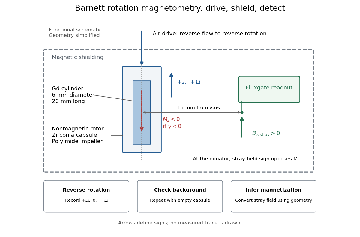
An additional analysis check follows from rotation symmetry. For signed sensor output , separateAn ideal linear Barnett effect appears in the odd component; a fixed offset appears in the even component. This is a proposed diagnostic, not a claim about the paper's processing. A background correlated with direction can also be odd: reversal alone is insufficient. Empty-rotor checks, zero-speed readings, calibration of sensor polarity, and controlled temperature changes test different errors. Equatorial stray-field sign must also be converted to magnetization sign: for an axial magnetic dipole moment, the magnetic dipole field at its equator points opposite to that magnetic moment. The apparatus diagram makes this otherwise easy-to-miss sign change visible.
The two-state calculation is not a general formula for a ferromagnet. Exchange interactions, magnetic domains, magnetic domain-wall pinning, magnetic anisotropy, and hysteresis can determine which response is accessible. Both spin angular momentum and orbital angular momentum can contribute; a single constant gyromagnetic ratio may be only a restricted effective description. Rotation sets an internal bias, while the material and its preparation determine magnetization. The Barkhausen effect illustrates why a smooth bias can produce jumps instead of the toy smooth curve.
For a limited, reversible, isotropic linear model, suppose the same intrinsic volume magnetic susceptibility responds to the applied bias and to . For a uniformly magnetized ellipsoid along a principal axis, include its demagnetizing factor :Solving this linear equation yieldsHere and are actual magnetic field intensities; the added rotational bias is an equivalent drive in the constitutive response. In SI, dimensionless multiplies an intensity in , so would omit and have the wrong units. A susceptibility defined instead as has different units. State the convention before comparing formulas.
At zero applied magnetic field intensity, a stipulated gives prefactor in a sphere, with , and a prefactor approaching in a long axial ellipsoid. This is a geometry check of the assumed linear model. A real cylinder does not have an exactly uniform demagnetizing field, and an irreversible ferromagnet cannot in general be represented by this single linear equation. Inferring an intrinsic gyromagnetic ratio requires an independently calibrated material response and a geometry-dependent conversion of the measured stray magnetic field.
Consider an explicitly stipulated dilute independent spin-one-half two-level system with zero applied magnetic field. Each constituent has and , with constant signed gyromagnetic ratio . Ignore interactions and the specimen's own magnetic field. At positive temperature , thermal equilibrium with the rotating lattice gives energy levels . Define the dimensionless variable , where is the reduced Planck constant and is the Boltzmann constant. The partition function and Boltzmann distribution giveTaking the expected value giveswhere is number density. This is the rotational version of the independent-moment magnetic response. The angular momentum aligns with positive rotation even when the magnetic moment points oppositely. The probability ratio provides a direct population check of the sign.
For , expand the hyperbolic tangent to obtainThe slope against is positive for either sign of , while the slope against has the sign of . At fixed , reversing reverses both means, and gives zero. At fixed nonzero , the formal limit saturates at ; the linear approximation must not be extrapolated there. At , the response vanishes. These limits describe the toy canonical ensemble, whose equilibration is assumed.
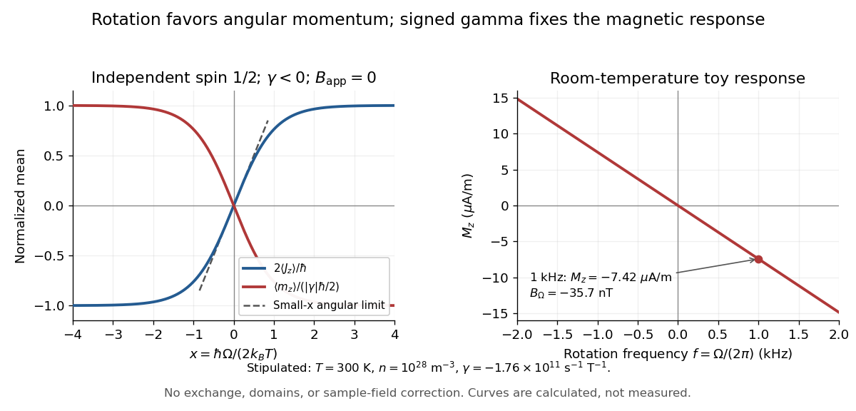
For a numerical example, stipulate , , , and rotation frequency . With , , and , the model givesThese are teaching inputs and calculated outputs, not measured material values. The corresponding internal angular momentum density is . Keeping a rotor at prescribed while its internal angular momentum changes requires the drive to supply the appropriate angular impulse. In an isolated body the mechanical part instead changes oppositely, as in magnetomechanical angular momentum balance. There is no creation of net angular momentum by choosing a rotating frame.
Let the specimen rotate uniformly with angular velocity . In its rotating reference frame, the internal Hamiltonian containsHere is the internal angular momentum operator about the rotation axis, and contains the internal interactions and any imposed magnetic field expressed in that frame. It does not include the separately treated rigid body's rotational kinetic energy. For a sector with magnetic moment , the rotational term has exactly the form of a magnetic dipole potential energy:This Barnett equivalent magnetic field has tesla units, with the angular convention for the signed gyromagnetic ratio: is in radians per second, not revolutions per second. Its sign matters. For an electronic contribution with , positive favors positive and negative . A sector with has the opposite magnetic sign. Equal need not correspond to equal Barnett fields for sectors having different gyromagnetic ratios.
A short derivation fixes the sign independently of any material model. Put and transform a laboratory quantum state by . The Schrödinger equation givesThe transformed laboratory term is denoted by ; a laboratory perturbation not stationary in the rotating frame can make it time dependent. Establishing a steady thermal response also requires exchange of internal angular momentum with the rotating body, for example through spin-lattice relaxation. A mere relabeling of coordinates cannot polarize isolated, unrelaxed spins.
The Barnett field is a useful description of spin-rotation coupling, not a claim that empty laboratory space acquires a uniform magnetic flux density . In particular, inserting it into the Lorentz force on an unrelated test electric charge is unjustified. A nearby magnetometer detects the specimen's actual stray magnetic field and backgrounds, rather than directly detecting this internal Hamiltonian parameter.
A hybridization gap is a separation in electronic band structure caused by mixing orbital-derived states. For , , and constant coupling , the lower eigenvalue is everywhere below and tends to it as . The upper eigenvalue has minimum . The unbounded model therefore has an indirect gap of width , approximately at weak coupling. This differs from the direct separation at the bare crossing. A finite Brillouin zone bounds the lower band farther below .
For two isotropic electron-like bands with equal spin degeneracy, conserving total carrier density conserves the sum of their occupied momentum-space volumes. If both uncoupled radii equal ,Only when the upper pocket is empty does this imply a single Fermi wavevector ; a nonzero mixing matrix element alone does not imply that emptying.
For a counterexample at arbitrarily weak coupling, take , , , and . At the uncoupled chemical potential , both pockets have radius . Let and . The characteristic equation at the Fermi level becomesFixed density cancels the first-order chemical-potential shift. Thus and : both pockets remain occupied at small coupling. This expansion assumes fixed before taking .
Mix a parabolic energy band with a perfectly flat band at through momentum-independent . At zero coupling suppose the two orbital sectors have equal populations, with the dispersive sector filled to . At fixed total density and sufficiently low temperature, nonzero coupling fills only the monotonic lower hybridized branch, whose Fermi wavevector is , provided the available momentum-space states accommodate it. Its small slope at that radius gives the displayed ratio to for . The result uses the singular perfectly flat limit and an empty upper band; it is not implied by Fermi-volume conservation in two hybridized electron bands for arbitrary pairs of dispersive bands. The zero-temperature limit must resolve the small hybridization energy scale.
Pinned article: Introduction to the OurBigBook Project
Welcome to the OurBigBook Project! Our goal is to create the perfect publishing platform for STEM subjects, and get university-level students to write the best free STEM tutorials ever.
Everyone is welcome to create an account and play with the site: ourbigbook.com/go/register. We belive that students themselves can write amazing tutorials, but teachers are welcome too. You can write about anything you want, it doesn't have to be STEM or even educational. Silly test content is very welcome and you won't be penalized in any way. Just keep it legal!
Intro to OurBigBook
. Source. We have two killer features:
- topics: topics group articles by different users with the same title, e.g. here is the topic for the "Fundamental Theorem of Calculus" ourbigbook.com/go/topic/fundamental-theorem-of-calculusArticles of different users are sorted by upvote within each article page. This feature is a bit like:
- a Wikipedia where each user can have their own version of each article
- a Q&A website like Stack Overflow, where multiple people can give their views on a given topic, and the best ones are sorted by upvote. Except you don't need to wait for someone to ask first, and any topic goes, no matter how narrow or broad
This feature makes it possible for readers to find better explanations of any topic created by other writers. And it allows writers to create an explanation in a place that readers might actually find it.
Figure 1. Screenshot of the "Derivative" topic page. View it live at: ourbigbook.com/go/topic/derivativeVideo 2. OurBigBook Web topics demo. Source. - local editing: you can store all your personal knowledge base content locally in a plaintext markup format that can be edited locally and published either:This way you can be sure that even if OurBigBook.com were to go down one day (which we have no plans to do as it is quite cheap to host!), your content will still be perfectly readable as a static site.
- to OurBigBook.com to get awesome multi-user features like topics and likes
- as HTML files to a static website, which you can host yourself for free on many external providers like GitHub Pages, and remain in full control

Figure 2. You can publish local OurBigBook lightweight markup files to either OurBigBook.com or as a static website.
Figure 3. Visual Studio Code extension installation.
Figure 5. . You can also edit articles on the Web editor without installing anything locally. Video 3. Edit locally and publish demo. Source. This shows editing OurBigBook Markup and publishing it using the Visual Studio Code extension. 
- Infinitely deep tables of contents:




All our software is open source and hosted at: github.com/ourbigbook/ourbigbook
Further documentation can be found at: docs.ourbigbook.com
Feel free to reach our to us for any help or suggestions: docs.ourbigbook.com/#contact