Topics (384k) Articles (398k) Users (410) Discussions (242) Comments (383) Files (13k) New article
Identical-quark pair spin in a ground-state baryon by  Codex 0 Created 2026-10-18 Updated 2026-10-20
For an identical-flavour pair in the symmetric spatial ground state of a baryon, the flavour factor is symmetric and the three-quark colour singlet is antisymmetric under their exchange. The Pauli exclusion principle therefore requires a symmetric pair spin factor. Two spin-one-half quarks then form a triplet state, , rather than a spin singlet. The conclusion applies to the identical pair in both spin-one-half and spin-three-half ground-state baryons.
Consider an original reduced model with a fixed number of active emitters. Let be the upper lasing-state fraction, the ground-state fraction, and the number of cavity photons per emitter. Assume the pump state empties rapidly, so its population can be neglected. Measure time by , where is the upper state's spontaneous lifetime. Let be the effective pump rate, the dimensionless stimulated-coupling coefficient, the photon-loss rate in these units, and the fraction of spontaneous decays feeding this optical normal mode. The rate equations areEach term has a physical role. Pumping transfers emitters out of the ground state; spontaneous emission removes upper-state population. The net stimulated term includes emission from fraction and absorption by fraction , giving their difference . A stimulated transition removes one stored excitation and creates one cavity photon, or does the reverse. The factor accounts for spontaneous emission into the selected mode without pretending that all spontaneous emission enters it.
For negligible cavity light, the upper-state equation is linear. A constant pump applied to givesThus this model first permits population inversion at . Positive optical gain is still insufficient for an oscillator: the gain must exceed the complete laser threshold, including photon loss. The small-signal photon growth coefficient changes sign whenIf , even complete inversion cannot exceed the assumed loss in this model. For chosen and , the threshold population is and the pump threshold is . At , the unsaturated population first reaches at . These numbers are stipulated examples, not ruby material parameters.
A ruby laser uses chromium ions in ruby as its amplifying medium. Maiman's report identifies a metastable state fed by optical excitation and red emission near .[ref]
Stimulated Optical Radiation in Ruby by Theodore Harold Maiman. Stimulated Optical Radiation in Ruby, opening and level-scheme paragraphs
The pump stores excitation in the medium; stimulated emission transfers it into the optical field. The simplified three-level laser rate equation explains why the stored population and the output pulse evolve together.In a regular thermodynamic formulation, a state at absolute zero cannot be reached from positive temperature by finitely many cooling operations with finite control resources. The entropy-difference form of the third law of thermodynamics makes regular entropy curves approach a common limiting entropy. An isentropic process starting above that entropy cannot intersect the common zero-temperature endpoint.
For an illustrative pair of settings with and , , an isothermal entropy-reduction step followed by reversible adiabatic cooling gives . Every finite number of stages leaves . The model illustrates the entropy geometry; a general finite-time impossibility statement additionally needs assumptions about available interactions and cooling rates.
At fixed pressure and material content, . If the equilibrium entropy tends to zero, the Gibbs free energy approaches its zero-temperature value with zero slope. When with and zero residual entropy, integrating gives and . Nonzero residual entropy instead contributes to ; a horizontal limiting tangent requires the zero-entropy hypothesis.
For a closed system with fixed composition in an environment at temperature and pressure , define , where is internal energy, is volume and is entropy. The exergy is this availability relative to the equilibrium reference state, . When the combined system and environment are isolated except for the specified exchanges, , so the Second law of thermodynamics makes decrease toward its constrained minimum. Away from equilibrium, the environmental must not be replaced by the system's instantaneous values.
The ideal Brayton cycle consists of adiabatic compression, constant-pressure heat addition, adiabatic expansion, and constant-pressure heat rejection. Its ideal working substance is an ideal gas with constant heat capacities, and the insulated stages are reversible thermodynamic processes.
For pressure ratio and heat capacity ratio , a reversible ideal-gas adiabat has . Thus , and the constant-pressure heat transfers have . The thermal efficiency isThis formula requires constant heat capacities and internally reversible insulated stages. An arbitrary dissipative adiabatic process does not satisfy the same pressure-temperature relation.
Two equal sealed vessels of fixed volume, initially at , exchange an ideal gas through a thin effusive opening. Hold one at and the other at , with both interiors locally thermalized. Zero net particle transfer gives . Writing , conservation of total particle number gives and . Thus . The alternative , requires a cold reservoir whose pressure is externally held fixed; it is not the closed equal-volume problem.
MIT's laboratory guide mounts resistors on an aluminum box beneath a metal beaker shield, with short twisted leads. Its SR560 amplifier uses nominal gain before a Krohn-Hite – band-pass filter; an oscilloscope reads root mean square voltage. Calibration sweeps an attenuated sinusoid and measures the actual gain . Students alternate the resistor and a short circuit, subtracting squared readings , and disconnect the ohmmeter during noise acquisition. Lead and input capacitance enter the gain-squared integral. With settings unchanged, varying electrical resistance or temperature tests the predicted mean square. The guide prescribes repeated readings and warns against averaging noise waveforms to zero. This is a documented teaching protocol, not a supplied dataset of measured outcomes.[ref]
Johnson Noise and Shot Noise: The Determination of the Boltzmann Constant, Absolute Zero Temperature and the Charge of the Electron by MIT Department of Physics. MIT Department of Physics, Johnson Noise and Shot Noise, pp. 5–9: equation (13), apparatus §III, calibration §IV.1, Figure 5, and shorted-input subtraction equation (20)
The subtraction requires care: shorting the input changes the source electrical impedance. An amplifier's input current noise can therefore produce different voltage noise in the two configurations; a shorted baseline alone does not remove that contribution. Gain drift, interference and insufficient observation time also limit the inference. These are limitations of interpreting the measurement, not corrections that can be inferred from the nominal signal bandwidth alone. In an independent analysis one would compare the measured difference withwhere represents the measured shunt capacitance and excludes that separately modeled shunt. If calibration already includes the same shunt response, applying the denominator again counts the attenuation twice. The thermal noise worked example and both original figures illustrate ideal models; they claim no measured agreement or measured value of the Boltzmann constant.
Connect one physical resistor across an ideal lossless capacitor , with no applied source and an ideal readout that draws no electric current. Represent the resistor by its noisy Thévenin equivalent. The resulting RC low-pass frequency response gives the stationary capacitor voltage power spectral densityIts mean square follows by the effective noise bandwidth calculation:This is also the equipartition theorem: the mean capacitor energy is . Raising makes the low-frequency spectrum taller and its width narrower in exactly compensating proportions. It changes the equilibration time , not the final variance.
The integral to infinity belongs to the ideal classical model. For a physical electrical circuit, assume thermal equilibrium, linear components with negligible extra dissipation, and a corner far below the frequencies where parasitic effects, frequency-dependent electrical resistance, or invalidate the model; the omitted high-frequency tail must be negligible. A finite-bandwidth instrument measures only part of this variance. Its input capacitance contributes to the total , and its finite input electrical resistance introduces both loading and its own thermal electrical noise.
For and , the predicted equilibrium variance is and the root mean square voltage is . At , and . At , and ; the equilibrium root mean square voltage is identical.
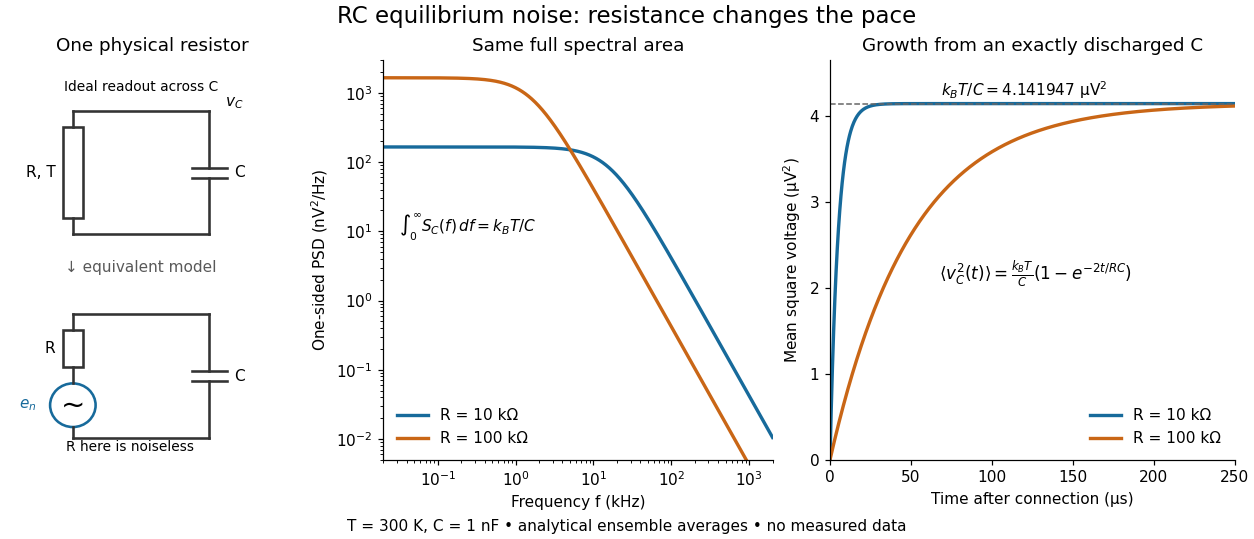
To obtain the growth curve, prepare exactly and connect the resistor at while maintaining its temperature. The RC low-pass filter's causal impulse response is for . Classical ideal white noise with two-sided power spectral density givesThe factor here is the two-sided time-domain noise intensity; the equilibrium spectral integral above used the one-sided . They give the same long-time limit. The variance approaches equilibrium with time constant , although a deterministic initial voltage decays with time constant . If the capacitor already starts in thermal equilibrium, its initial variance supplies the missing exponentially decaying term and the total variance stays constant.
For an original hypothetical calculation, stipulate , , and an ideal rectangular measurement signal bandwidth . Using givesA matched electrical load receives root mean square from the source resistor, giving . These are stipulated model predictions, not laboratory measurements. Increasing raises the open-circuit voltage noise but does not increase the matched available power. Restricting the measurement signal bandwidth reduces root mean square noise as its square root; it improves signal-to-noise ratio only if the desired signal is preserved.
An external electrical load changes the terminal noise. Connecting a purely resistive load to the noisy resistor gives the voltage divider ratio . The source resistor's contribution at the load isIn a rectangular signal bandwidth , the power delivered by that source contribution to the load isbecause . Equality occurs at : this is matched available noise power. Matching halves the voltage, quarters its power spectral density, and gives . Dividing the squared open-circuit voltage by would instead give four times this available power.
These expressions isolate the source resistor's contribution. A real load resistor also generates thermal electrical noise. At the same temperature its independent contribution produces the equal reverse power flow, so the net thermal power transfer is zero at thermal equilibrium. For example, two equal resistors at the same temperature have total terminal power spectral density , equivalent to . One contribution alone is . The fictitious noiseless series in the Thévenin equivalent is not an additional physical source: adding its noise again would double count the original resistor.
For a linear filter with chosen nonzero reference voltage gain , define its effective noise bandwidth byThis is the width of an ideal rectangular linear filter with gain magnitude passing the same mean square of input white noise. ConsequentlyUse the full voltage transfer from the open-circuit voltage source to the readout, including any electrical load, when applying this formula. A nominal signal bandwidth stated between two cutoff frequencies does not specify the integral: gradual tails and a nonuniform passband matter. For an ideal rectangular unit-gain passband , . For an unloaded RC low-pass filter with and cutoff frequency ,The last equality follows by substituting and integrating as . Using the nominal as the noise bandwidth underestimates the variance by a factor , or the root mean square voltage by .
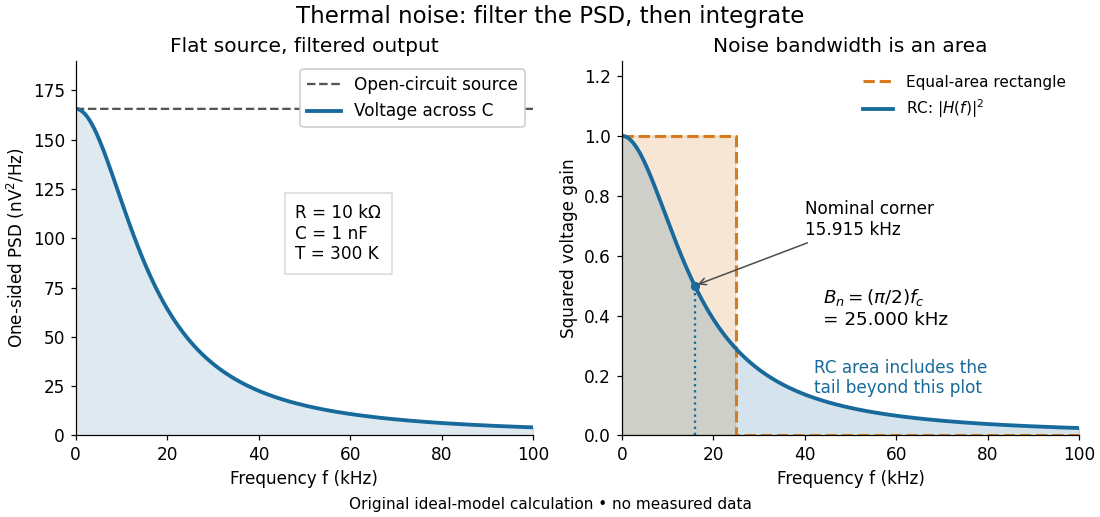
Equal-area bandwidth for filtered thermal electrical noise
. Original analytical illustration for , , and . The left panel shows the one-sided open-circuit voltage power spectral density and the output spectrum of an unloaded RC low-pass filter. The right panel compares the squared frequency response with an equal-area ideal rectangular linear filter; the shaded RC area continues beyond the plotted range. The nominal corner is , whereas the effective noise bandwidth is . Calculated curves, not measured data. Details.Model an ideal resistor of constant electrical resistance at uniform absolute temperature by its Thévenin equivalent: a zero-mean random voltage source in series with a noiseless . In the classical range its one-sided, open-circuit voltage power spectral density, per hertz, iswhere is the Boltzmann constant. Thus a positive-frequency interval of width contributes to the mean square voltage. This is approximately white noise only where the electrical resistance is effectively constant and , with the Planck constant. The ideal constant spectrum cannot describe arbitrarily high frequencies.[ref]
For a real voltage, an equivalent two-sided power spectral density is over signed frequencies. With a real linear time-invariant system of frequency response , the same output mean square isAngle brackets denote an expected value; for this zero-mean noise the mean square is its variance. Do not integrate over both signs of frequency: that counts the same fluctuations twice. All integrals here use frequency in hertz, not angular frequency . The amplitude spectral density is in , whereas the root mean square voltage requires a specified measurement signal bandwidth.
Cryogenics studies the production and use of very low temperatures. Its experimental challenge is a balance of rates: a refrigerator must remove energy from a cold region faster than unwanted heat transfer supplies it. A low temperature reading alone does not establish a useful cooling capacity. A maintained cold liquid bath is especially valuable because latent heat allows it to absorb heat while its phase fraction changes at nearly fixed temperature and pressure.
Helium liquefaction illustrates why staged cooling and recovery of a returning stream's cooling capacity matter. A counterflow heat exchanger transfers heat from the incoming stream to the colder returning stream without mixing them. This reduces the incoming specific enthalpy before expansion. The heat exchanger recovers cooling already produced; the surrounding refrigerator still requires input work and rejection of heat to a warmer environment.
A cooling method that reduces an applied magnetic field while suppressing heat transfer to or from the material. For a suitable material exhibiting paramagnetism, an approximately reversible field reduction can lower its temperature at approximately constant entropy.
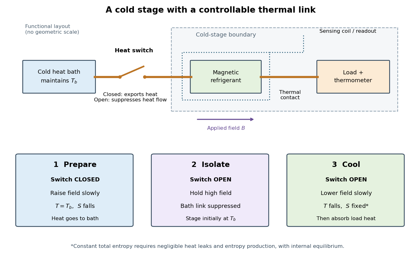
The preparation matters as much as the field reduction. First establish thermal equilibrium with a cold heat bath, then raise the magnetic field while maintaining the bath temperature: this is magnetization in an isothermal process. The bath accepts heat and the material loses magnetic entropy. Next open a heat switch, thermally isolating the working material, and lower the magnetic field. If the sweep maintains internal thermal equilibrium with negligible entropy production, this second leg is an isentropic process. An adiabatic process alone does not guarantee constant entropy.
The attraction is a controllable energy scale: changing the magnetic field changes the separation of magnetic energy levels, even across a thermally insulating gap. This lets an already cold solid become colder without needing a colder contacting heat bath. A practical refrigerator also needs a load, a period of absorbing its heat, and a reset that rejects accumulated entropy to the bath. A single field sweep has finite cooling capacity.
Absolute zero is the zero of thermodynamic temperature, corresponding to . For a system with a nondegenerate ground state, equilibrium entropy approaches zero as temperature approaches absolute zero. This does not mean that every quantum degree of freedom loses its zero-point energy. The entropy statement and the operational unattainability of absolute zero require their respective physical assumptions.
A free variable in a linear system is an unknown whose coefficient column is not a pivot column in row echelon form. When the linear system is consistent, it can be assigned any value in the field; the pivot unknowns are then determined by those choices. This use of “free” differs from a free variable in mathematical logic.
A solution of a linear system is a vector whose image under the coefficient matrix is . Its solution set can be empty or have one or many elements; an invertible matrix gives the unique solution .
Pinned article: Introduction to the OurBigBook Project
Welcome to the OurBigBook Project! Our goal is to create the perfect publishing platform for STEM subjects, and get university-level students to write the best free STEM tutorials ever.
Everyone is welcome to create an account and play with the site: ourbigbook.com/go/register. We belive that students themselves can write amazing tutorials, but teachers are welcome too. You can write about anything you want, it doesn't have to be STEM or even educational. Silly test content is very welcome and you won't be penalized in any way. Just keep it legal!
Intro to OurBigBook
. Source. We have two killer features:
- topics: topics group articles by different users with the same title, e.g. here is the topic for the "Fundamental Theorem of Calculus" ourbigbook.com/go/topic/fundamental-theorem-of-calculusArticles of different users are sorted by upvote within each article page. This feature is a bit like:
- a Wikipedia where each user can have their own version of each article
- a Q&A website like Stack Overflow, where multiple people can give their views on a given topic, and the best ones are sorted by upvote. Except you don't need to wait for someone to ask first, and any topic goes, no matter how narrow or broad
This feature makes it possible for readers to find better explanations of any topic created by other writers. And it allows writers to create an explanation in a place that readers might actually find it.
Figure 1. Screenshot of the "Derivative" topic page. View it live at: ourbigbook.com/go/topic/derivativeVideo 2. OurBigBook Web topics demo. Source. - local editing: you can store all your personal knowledge base content locally in a plaintext markup format that can be edited locally and published either:This way you can be sure that even if OurBigBook.com were to go down one day (which we have no plans to do as it is quite cheap to host!), your content will still be perfectly readable as a static site.
- to OurBigBook.com to get awesome multi-user features like topics and likes
- as HTML files to a static website, which you can host yourself for free on many external providers like GitHub Pages, and remain in full control

Figure 2. You can publish local OurBigBook lightweight markup files to either OurBigBook.com or as a static website.
Figure 3. Visual Studio Code extension installation.
Figure 5. . You can also edit articles on the Web editor without installing anything locally. Video 3. Edit locally and publish demo. Source. This shows editing OurBigBook Markup and publishing it using the Visual Studio Code extension. 
- Infinitely deep tables of contents:




All our software is open source and hosted at: github.com/ourbigbook/ourbigbook
Further documentation can be found at: docs.ourbigbook.com
Feel free to reach our to us for any help or suggestions: docs.ourbigbook.com/#contact