Topics (384k) Articles (398k) Users (410) Discussions (242) Comments (383) Files (13k) New article

Diffuse X-ray background is X-ray emission spread over the instrument's observed sky rather than assigned to a single resolved source. Diffuse appearance at finite angular resolution does not prove emission by a continuous medium: many unresolved point-like astronomical sources can also give a smooth signal. Instrumental background is a separate contribution, even though both enter measured counts.
In 1962, Riccardo Giacconi and colleagues flew three Geiger counters to search for lunar X-ray fluorescence. Different mica thicknesses tested penetration; lampblack blocked ultraviolet. Each counter sat in an anticoincidence detector using a scintillation counter to reject cosmic rays. There was no mechanical collimator. Rotation scanned the sky; optical sensors supplied orientation.[ref]
Evidence for x Rays From Sources Outside the Solar System by Riccardo Giacconi and others. pp. 439–440, apparatus and readout
Counts were sorted by azimuth; a faulty counter and tumbling descent data were excluded. A directional peak lay above a diffuse component. Window, altitude and angular responses tested X-rays against charged particles; the Moon's nondetection checked optical leakage. The authors argued for an origin outside the Solar system, while residual cosmic ray background was not directly measured and source size, position and spectrum remained assumption-dependent.[ref]
Evidence for x Rays From Sources Outside the Solar System by Riccardo Giacconi and others. pp. 440–443, Figs. 1–4 and concluding limitations
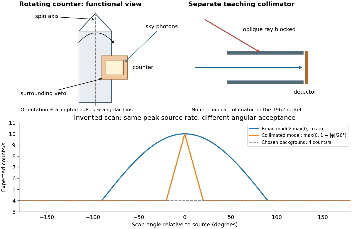
A simple original forward problem makes the distinction precise. Let be the scan azimuth, let be a dimensionless directional response with maximum one, let be a source's band-integrated photon arrival rate per unit area, let be its on-axis X-ray effective area, and let be a constant accepted background rate. The expected rate isFor a broad illustrative response , the full width at half maximum is : at . For a one-dimensional ideal collimator model , the full width at half maximum is . Choosing narrows the response sixfold without focusing any additional photons. These are teaching response functions, not reconstructions of the rocket's window transmission or geometry. A narrower scan peak can reflect the instrument response even when the source is unresolved.
A cosmic X-ray source is an astronomical emitter detected through its X-rays. Hot plasma, energetic particles and matter falling into deep gravitational potentials can produce such radiation, so detection alone does not identify a black hole or one unique emission mechanism.
A useful observation proceeds from an excess of detector events to a sky location, spectrum and light curve. Background rejection and response calibration determine which incident photons could have produced those events. The 1962 rocket discovery of cosmic X-ray sources illustrates how a scanning detector and an independent orientation measurement can establish a celestial signal without forming an ordinary optical image.
Radiography forms an image from spatially resolved transmission of X-rays or other penetrating radiation. A source illuminates the object, and a detector on the other side records how much radiation reaches each position. Variations in attenuation make internal differences observable without cutting the object.
A thicker region and a more strongly absorbing material can give similar transmission, so one projection does not uniquely determine composition or three-dimensional shape. Unwanted scattering reduces image contrast by adding radiation that did not follow the intended straight path. A reference exposure measures source and detector nonuniformity; multiple viewing directions provide additional geometric information.
For a narrow beam of monoenergetic photons crossing homogeneous material of thickness , the uncollided wave intensity obeys . Here is the linear attenuation coefficient, counting removal from the incident beam by photon absorption and scattering of light. It depends on photon energy and material; it is not universally independent of energy.[ref]
2. The Mass Attenuation Coefficient. Tables of X-Ray Mass Attenuation Coefficients and Mass Energy-Absorption Coefficients by John H. Hubbell and Stephen M. Seltzer; NIST, X-Ray Mass Attenuation Coefficients, §2, Eq. (1), narrow monoenergetic beam and interaction contributions
An original derivation makes the model explicit. If each thin layer removes fraction of the surviving beam, with the same throughout, thenThus equal added thicknesses multiply transmission by the same factor. The ordinary differential equation describes uncollided beam survival. To test it with a detector, keep source output, distance, selected photon energy band and detector response fixed. Use a collimator and suitable detector acceptance to exclude scattering of light into the detector. Subtract background, measure an empty-path reference, and keep the detector in its linear operating range. A changing source distance adds geometric dilution and is not an attenuation measurement at fixed geometry.
For a stipulated example, take and . Transmission is . If the empty-path detector rate is , including background , the model predicts sample rate . Recover transmission as ; the raw ratio is biased. These chosen values are a calculation, not measurements of a particular material or a historical apparatus.
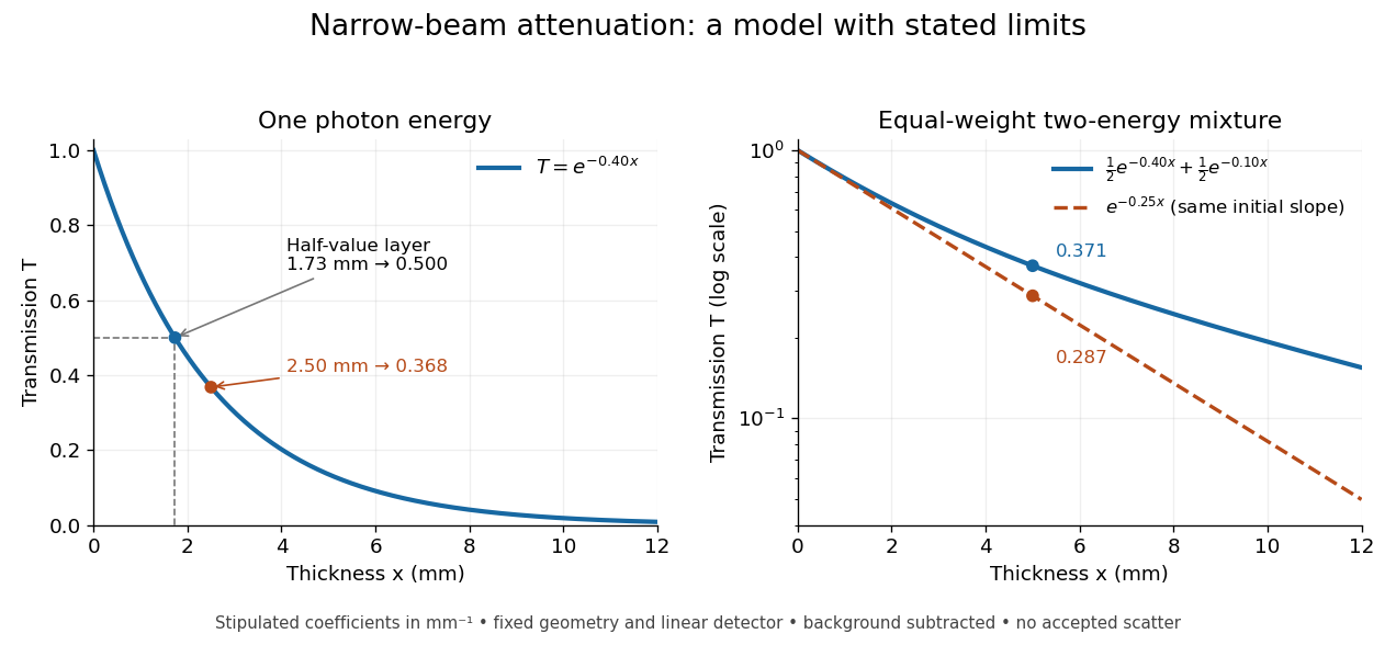
When X-ray transmission is exponential, and when spectral mixing bends it
. Original calculated examples, with stipulated linear attenuation coefficients in inverse millimetres. The left panel uses one photon energy and marks and the half-value layer. The right panel compares an equal-weight mixture of two photon energies with the exponential having the same initial slope. A logarithmic vertical axis turns a single exponential into a straight line. Neither curve is fitted to measured material data. Details.An X-ray tube accelerates electrons from a negative cathode to a positive target anode. A heated cathode supplies electrons by thermionic emission; the evacuated envelope limits collisions before the target. This differs from the gas-discharge tube in the Röntgen X-ray discovery experiment.[ref]
Chapter 5: X-Ray Production (teaching slides) by K. P. Maher. Diagnostic Radiology Physics: A Handbook for Teachers and Students; IAEA, Chapter 5: X-Ray Production, §§5.2–5.3.2; authored teaching slides, inspected transcription
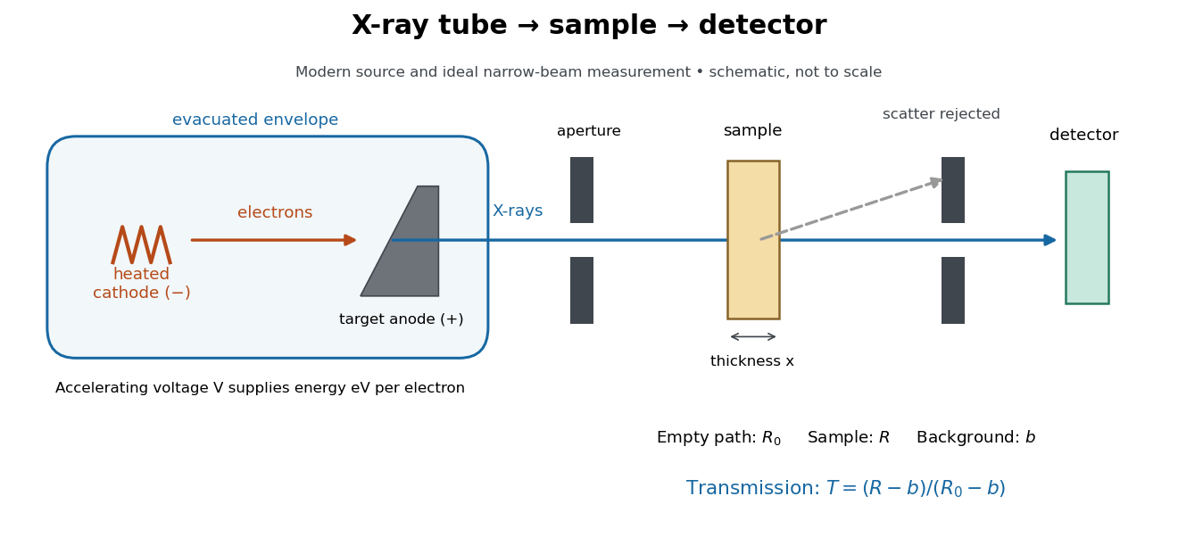
In bremsstrahlung, an electron changes velocity in the target's electric fields, emitting a photon while losing kinetic energy. Different encounters allow a continuous range of transferred energies. This is distinct from the discrete electronic transitions producing Characteristic X-rays.
Changing the accelerating voltage changes the available kinetic energy per electron and the X-ray tube cutoff. Changing the number of arriving electrons changes the number of opportunities for photon emission. These are distinct controls: a larger electric current does not by itself give each electron more energy. For an original idealized budget, and tube electric current give electrical power and arrival rate , where is the elementary charge. This is input power, not emitted X-ray power; obtaining the latter requires a conversion efficiency.
In 1924–1925, Walther Bothe and Hans Geiger tested event-level Compton scattering correlations against the statistical conservation proposed by BKS theory.[ref]
The Coincidence Method by Walther Bothe. The coincidence method, pp. 271–273
Needle Geiger counters shared a wall. X-rays passed beside it through hydrogen; recoil electrons registered in one counter and scattered photons triggered electron release in the other. Photographic records resolved approximately .[ref]
The Coincidence Method by Walther Bothe. p. 272: apparatus and timing
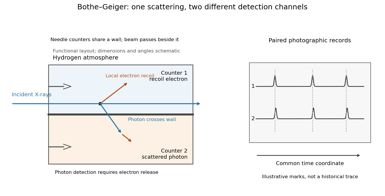
Two detection channels in the Bothe-Geiger coincidence experiment
. Original functional schematic based on Bothe's account; dimensions, angles and trace marks are illustrative. The common wall separates the counter regions; the direct beam avoids it. The drawing specifies neither wall material nor chamber shape. Photon detection requires electron release. Both records share a time coordinate. Details.The coincidence excess matched paired-emission expectations. Bothe distinguishes a later directional test from this timing experiment.[ref]
The two channels have different physical roles. The first responds to the local recoil electron's ionization. The second converts a scattered photon into an electron response, as in the photoelectric effect. A large counter signal is an amplified indication of an interaction, not a direct measurement of the incoming photon's energy. The detection efficiency and accepted directions determine how many genuine partners can be seen. Consequently, failure to record every partner is compatible with paired production.
The relevant distinction is between an average balance and a balance in each event. For an initially stationary free electron, Compton recoil kinematics givesHere are incident and scattered photon energies, is recoil kinetic energy, and is electron momentum. These are paired constraints, not just equations between averages over unrelated detections. Summing correctly paired events preserves the equations; throwing away the pair identities loses information. Two samples can have identical separate energy distributions while differing in their joint probability distribution.
The experiment therefore supplied evidence for the event association required by photon recoil, rather than weighing both outgoing energies in every event. A statistically established excess above accidental coincidences matters; one near-simultaneous pair cannot establish the association. It also cannot by itself settle every question about wave-particle duality.
Preparation, readout and background checks address different failure modes. The direct beam must avoid the second counter, and the counter boundary must prevent a recoil electron from masquerading as its own photon partner. Separate-channel rates constrain accidental coincidences; common disturbances or electrical coupling could instead create a correlated instrumental background. A useful diagnostic is to displace one record in time: under a stationary process assumption, unrelated-pair expectations persist while prompt partners separate. This is the explanatory control modeled below, not an assertion that Bothe performed that particular record-shifting procedure. A background estimate and a statistical comparison are essential to the inference.
The existing coincidence circuit article explains electronic selection, and accidental coincidence derives the accepted-window background. Here pairing can be understood directly from the two recorded time sequences, without imposing a modern detector trigger on the historical readout.
Wilhelm Conrad Röntgen's 1895 first communication describes an induction coil driving an evacuated gas-discharge tube, enclosed in black cardboard in darkness. A paper screen coated with barium platinocyanide showed fluorescence even with its uncoated side facing the tube, visible two metres away. The covering excluded ordinary illumination.[ref]
On a New Kind of Rays by Wilhelm Conrad Röntgen. Röntgen, On a New Kind of Rays, §§1–2; inspected reprint p. 153
He interposed materials: a thousand-page book transmitted; lead was practically opaque. A stepped stack of foil produced a photographic plate record. Different materials were not equivalent at equal density and thickness. Photographic plates checked visual observations while remaining covered against ordinary illumination.[ref]
On a New Kind of Rays by Wilhelm Conrad Röntgen. First communication, §§2–6; reprint pp. 153–154: absorption tests and photographic controls
Section 14 lists photographs of hand bones, wire on a bobbin, boxed weights, an enclosed compass, and a lead-painted door. It does not identify the hand's owner. Magnetic deflection moved the cathode ray impact point and thus the source, without bending the emerging X-rays. Their nature remained unsettled.[ref]
On a New Kind of Rays by Wilhelm Conrad Röntgen. First communication, §§11–14 and 17; reprint pp. 156–157
The observations belong to 1895; the contemporary English translation appeared in Nature on 23 January 1896.[ref]
On a New Kind of Rays by Wilhelm Conrad Röntgen. Catalogue, On a new kind of rays: notes identify the Nature translation and its publication date
The experimental logic separates production, transmission and detection. A visibly opaque covering can transmit X-rays; fluorescence then converts deposited energy into visible light. A shadow measures a difference between paths through an object, rather than a direct view of its surface. Neither a screen's brightness nor photographic darkness alone measures an absolute X-ray energy or establishes the X-ray attenuation law below.For a free three-dimensional worm-like chain with contour length and persistence length , the unit-tangent correlation is . Since , integrating this correlation givesFor , the leading term is , the ideal chain law with Kuhn length . For , a Taylor series gives , approaching a rigid rod. This ideal semiflexible-chain model omits long-range excluded volume; sufficiently long dilute chains in a good solvent can cross over to swollen-chain statistics.
Multiplying a measured signal by a finite-duration window function convolves its Fourier transform with the transform of the window. A spectrally sharp component therefore contributes to nearby frequencies rather than remaining a single ideal line. Smooth tapering can reduce distant sidelobes at the cost of widening the main spectral feature. This finite-record effect is distinct from aliasing, which superposes copies of the spectrum because of time sampling.
Use the equal-component Wien bridge with upper-left parallel arm and lower-left series arm. Let be the left arm junction, the upper input node, and the upper-minus-lower input electric potential difference. With , the unloaded transfer ratio is the displayed expression. Its band-pass filter magnitude is , maximal at with . One continuous wave phase is , tending from at low positive frequency to at high frequency. Reversing the measured output polarity multiplies by and shifts its phase by without changing its magnitude.
A Cassie–Baxter state is a composite wetting state in which a drop contacts solid asperities over area fraction and trapped gas over the remainder. An ideal area-weighted contact-angle model gives the displayed apparent angle from the smooth-solid Young's equation angle . Reducing solid contact can strongly enhance apparent hydrophobicity. Such a state can be metastable and can collapse when liquid enters the texture; roughness alone does not guarantee it.
The excess interfacial free energy released per newly wetted area when a liquid film replaces a solid-vapour interface is the displayed coefficient. Positive favors macroscopic spreading in the ideal equilibrium surface-energy model, whereas negative permits a finite contact angle obeying Young's equation. Surface preparation, chemical composition and adsorption can change all three interfacial energies.
A liquid spreads macroscopically over a solid with zero macroscopic equilibrium contact angle. In the simple interfacial-energy model the threshold is , or zero spreading coefficient; positive coefficient favors a spreading film. Extrapolating a concentration-dependent liquid-vapour surface tension to this threshold assumes the other interfacial energies remain fixed and no intervening adsorption or micellization behavior changes the trend.
For and positive temperature, the positive solution exists uniquely for : the slope at zero is , while the hyperbolic tangent is concave and below one. For only remains. Expanding to cubic order near gives and , with mean-field critical exponent . The prefactor follows from the truncated equation; it is not controlled beyond leading critical order.
Parity violation means that a physical law fails to be invariant under the spatial reflection represented by the parity operator. A process and its fully inverted counterpart can then have different probabilities. For beta-minus decay with polarized parent atomic nuclei, a nonzero correlation between nuclear spin and emitted electron momentum is such a test. Rotational symmetry alone allows this correlation: a pseudoscalar is unchanged by proper rotations but changes sign under spatial reflection.
A decay amplitude changing strangeness by two units requires at least two insertions of the low-energy weak interaction in the Standard Model. Each charged-current insertion can remove only one net strange quark in such a process. Both two-W boson tree topologies and loop contributions can occur; a loop is not required for every exclusive final state. At hadronic energies, the extra power of the Fermi constant, with the needed powers of an energy scale to balance units, strongly suppresses a second-order amplitude relative to a first-order one. This is distinct from Cabibbo suppression within a fixed weak order.
In a low-energy allowed weak three-body decay, negligible final-state masses and a nearly constant effective matrix element give a fifth-power energy-release dependence. For muon decay in natural units, . This four-fermion approximation requires momentum transfers small compared with the W boson mass. Extrapolation to a heavy particle able to emit a real W changes the decay kinematics and the mass scaling, so it is not a reliable heavy-particle lifetime prediction.
For equal-mass one-dimensional scattering between regions with real wavenumbers , insert a layer of width and wavenumber . For a purely right-moving incident wave of amplitude and no reflection, continuity at the first edge gives interior amplitudes and . If , continuity at the second edge gives a transmitted edge amplitude and the matching condition . Thus and the transmitted probability current equals the incident current, despite their unequal amplitudes.
For potentials with , the condition is , or , requiring . It is the quantum-wave counterpart of a quarter-wave impedance transformer: the intermediate wavenumber is the geometric mean and the two reflected amplitudes cancel.
Anderson localization is the confinement of electron wave functions, or other wave modes, by interference between repeated wave scattering paths in static disorder. A localized eigenstate occupies a limited region even in a much larger sample. Disorder can therefore suppress diffusion without absorbing the wave. In 1958, Philip Warren Anderson studied random site energies and intersite coupling, finding a regime without transport. His paper develops a theoretical model; it does not report an Anderson laboratory measurement.[ref]
Absence of Diffusion in Certain Random Lattices by Philip Warren Anderson. Anderson, 1958, pp.1492–1494, Sections I–II
The distinction from ordinary multiple scattering is the retention of wave phases: alternative paths contribute probability amplitudes before their squared modulus is taken. Adding path probabilities alone loses the cross terms responsible for interference. This makes Anderson localization useful as a warning about transport models: repeated deflections need not produce unlimited diffusion. It also connects electron transport with wave propagation in a random medium, although the detailed equations and experimental diagnostics differ between electrons, light and acoustic waves.
Philip Warren Anderson's 1977 lecture distinguishes localized magnetic moments from disorder-localized states. It credits Nevill Francis Mott with recognizing the significance of the mobility edge. A Mott insulator instead requires electron interactions and can exist without disorder.[ref]
Local Moments and Localized States by Philip Warren Anderson. Local Moments and Localized States, pp.376–377,395–396; inspected institutional mirror www.nevis.columbia.edu/~haas/documents/physics_nobel_lectures/physics71-80-2.pdf
John Hasbrouck Van Vleck developed quantum mechanics explanations of magnetic susceptibility, including its temperature dependence; this is a distinct contribution from Anderson localization.[ref]
Quantum Mechanics: The Key to Understanding Magnetism by John Hasbrouck Van Vleck. Quantum Mechanics: The Key to Understanding Magnetism, pp.355–356; inspected institutional mirror www.nevis.columbia.edu/~haas/documents/physics_nobel_lectures/physics71-80-2.pdf
Pinned article: Introduction to the OurBigBook Project
Welcome to the OurBigBook Project! Our goal is to create the perfect publishing platform for STEM subjects, and get university-level students to write the best free STEM tutorials ever.
Everyone is welcome to create an account and play with the site: ourbigbook.com/go/register. We belive that students themselves can write amazing tutorials, but teachers are welcome too. You can write about anything you want, it doesn't have to be STEM or even educational. Silly test content is very welcome and you won't be penalized in any way. Just keep it legal!
Intro to OurBigBook
. Source. We have two killer features:
- topics: topics group articles by different users with the same title, e.g. here is the topic for the "Fundamental Theorem of Calculus" ourbigbook.com/go/topic/fundamental-theorem-of-calculusArticles of different users are sorted by upvote within each article page. This feature is a bit like:
- a Wikipedia where each user can have their own version of each article
- a Q&A website like Stack Overflow, where multiple people can give their views on a given topic, and the best ones are sorted by upvote. Except you don't need to wait for someone to ask first, and any topic goes, no matter how narrow or broad
This feature makes it possible for readers to find better explanations of any topic created by other writers. And it allows writers to create an explanation in a place that readers might actually find it.
Figure 1. Screenshot of the "Derivative" topic page. View it live at: ourbigbook.com/go/topic/derivativeVideo 2. OurBigBook Web topics demo. Source. - local editing: you can store all your personal knowledge base content locally in a plaintext markup format that can be edited locally and published either:This way you can be sure that even if OurBigBook.com were to go down one day (which we have no plans to do as it is quite cheap to host!), your content will still be perfectly readable as a static site.
- to OurBigBook.com to get awesome multi-user features like topics and likes
- as HTML files to a static website, which you can host yourself for free on many external providers like GitHub Pages, and remain in full control

Figure 2. You can publish local OurBigBook lightweight markup files to either OurBigBook.com or as a static website.
Figure 3. Visual Studio Code extension installation.
Figure 5. . You can also edit articles on the Web editor without installing anything locally. Video 3. Edit locally and publish demo. Source. This shows editing OurBigBook Markup and publishing it using the Visual Studio Code extension. 
- Infinitely deep tables of contents:




All our software is open source and hosted at: github.com/ourbigbook/ourbigbook
Further documentation can be found at: docs.ourbigbook.com
Feel free to reach our to us for any help or suggestions: docs.ourbigbook.com/#contact