Topics (384k) Articles (398k) Users (410) Discussions (242) Comments (383) Files (13k) New article
A point measure is a countable sum of Dirac measures. It is simple if all its atoms have mass one, and locally finite if every bounded set has finite mass. Simplicity lets fine enough cells count individual points, whereas occupation indicators would lose multiplicities in a nonsimple measure.
The void probability functional assigns to a measurable set the probability that it contains no atom of a random point measure. For a Poisson random measure of intensity , it is . The exponential void probabilities characterize a Poisson random measure result uses simplicity; doubling every atom of a Poisson measure preserves void probabilities but changes count distributions.
The intensity measure of a point process is its expected counting measure:It may take the value .[ref]
Lectures on the Poisson Process by Günter Last and others. Section 2.2, Definition 2.5, printed p. 12: intensity as the expected counting measure
Countable additivity follows by applying the monotone convergence theorem to the counts of finite unions of pairwise disjoint observation windows. If is locally finite and absolutely continuous with respect to Lebesgue measure, its Radon-Nikodym derivative is the intensity function of a point process :This is an expected number per unit volume, not a probability density function for a randomly selected point. For example, a single deterministic point has , a Dirac measure, and no Lebesgue measure density. The density representation requires its own assumption.[ref]Spatial Point Processes and their Applications. Section 2.1, Definitions 2.1-2.2, printed pp. 26-27: expected counts and intensity functions
For a bounded Borel set , , but local finiteness alone does not ensure that this expected value is finite. Conversely, implies almost surely, even when is unbounded. A constant finite intensity function of a point process on all of has infinite total intensity measure, although every bounded window has finite expected value.
A Neyman-Scott process places independent offspring clusters around points of a Poisson parent process, with an independently drawn offspring count and displacements. Poisson offspring counts make the offspring process conditionally Poisson given the parents, and therefore give a Cox process. Arbitrary offspring counts need not have that property.
A point process on is stationary if every translation preserves its probability law. If its mean count in a unit cube is finite, its intensity measure is for some , where denotes Lebesgue measure. This follows because stationarity makes the mean measure invariant under translations. A constant intensity function of a point process describes only these mean counts, and by itself asserts neither stationarity of the entire law nor independence.[ref]
Lectures on the Poisson Process by Günter Last and others. Section 8.1, Proposition 8.2, printed pp. 69-70: stationarity and constant intensity under a finite unit-cube mean
For a bounded Borel set , the window count of a locally finite point process is a finite nonnegative integer random variable. It counts multiplicities, and the convention for window boundaries matters. On the time half-line, is a counting process and . For pairwise disjoint observation windows , the measure identityis valid for every realization. Additivity of counts supplies no independence assumption.
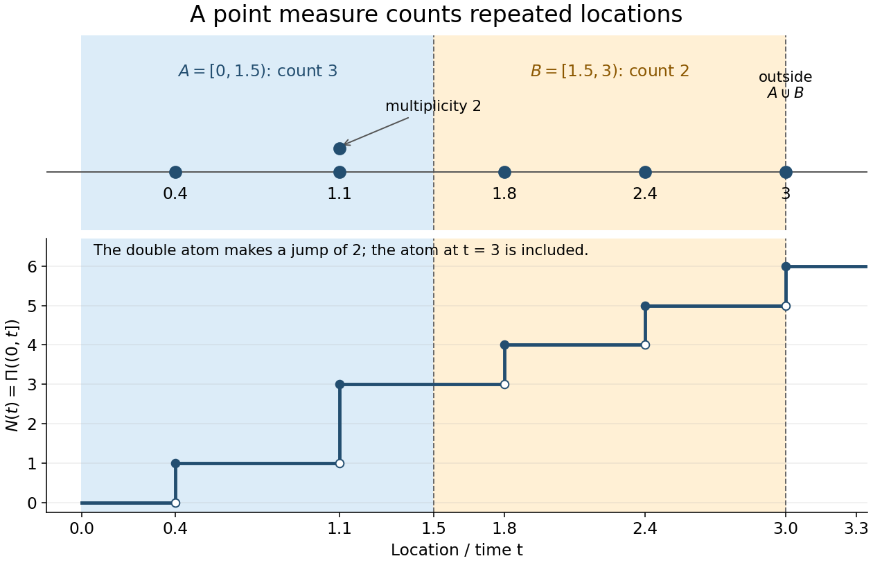
Window counts include multiplicity and depend on boundary conventions
. One locally finite point measure is . The half-open windows and have counts three and two; . The atom at three lies outside both windows. Two stacked dots denote the double atom at , and the step plot records , which includes the atom at three. Details.A point process is simple when, on a single almost sure event, every location has multiplicity at most one. Its realizations are simple locally finite point measures. For instance, is locally finite but not simple: it has four points counted with multiplicity at three distinct locations. Simplicity is a statement about each entire realization. Checking separately for every fixed is insufficient: with having the uniform distribution on passes every such fixed-location check, yet always has a double point.[ref]
Lectures on the Poisson Process by Günter Last and others. Section 6.2, Definitions 6.6 and 6.8, printed p. 49: simple measures and simple point processes
The boundary of a chosen Poincare coordinates on anti-de Sitter spacetime patch inside the full spacetime is a null coordinate horizon. It is not the timelike conformal boundary, and not a curvature singularity. Timelike geodesics can cross it in finite proper time while the patch time diverges. In a signed-diameter conformal strip, the patch containing satisfies .
For unit-radius metric , translations conserve . Timelike normalization gives and . Setting yields , hence the displayed proper-time solution where the cosine is positive. Its two patch-horizon crossings are separated by proper time , although the globally extended geodesic is complete.
An astronomical conjunction occurs when two orbiting bodies have the same apparent longitude as viewed from their primary or from an observer.
A planetary dynamo maintains an intrinsic magnetic field by motion of an electrically conducting fluid. The resistive induction equation balances stretching and transport against magnetic diffusion. A sufficiently large magnetic Reynolds number is necessary but does not ensure that the flow regenerates every required field component. Thermal or compositional convection supplies mechanical power; rotation organizes the flow through the Coriolis force, and the Lorentz force density eventually modifies the flow and limits growth. A fluid core can fail to operate a dynamo if it is stably stratified or inadequately driven.
The innermost planet has a large metallic core and a weak but global intrinsic magnetic field. Its observed field supports an active planetary dynamo in a fluid conducting part of that core. Slow rotation does not by itself exclude dynamo action.
Two viscous layers occupy and , with viscosities and . A uniform driving pressure gradient , a stationary flat interface and no-slip outer walls give the displayed plane Poiseuille flow, where and . These constants follow from continuity of velocity and shear stress at the interface and zero wall velocities. The upper-to-lower volume-flux ratio is , with . As , the interface becomes effectively stationary, the upper flux vanishes, and the lower layer approaches flow between two stationary plates a distance apart. The upper wall stress remains finite despite its vanishing velocity gradient.
Symmetric viscous interaction in an indented Poiseuille channel by  Codex 0 Created 2026-10-14 Updated 2026-10-20
At large Reynolds number , a long indentation of relative height has nonlinear near-wall interaction when the streamwise scale ratio satisfies . The regime gives a thin viscous layer and an effectively common pressure across the core. The core displacement is and . A lower wall displaced to produces layer displacement , while the upper wall produces . Uniqueness for their common pressure forcing and upstream data makes the two layer displacements equal, so .
A steady planar viscous jet whose conserved momentum flux and convection-diffusion balance give the displayed scaling. Choosing and as centre-line speed gives streamfunction profile , with , and . Integration yields and velocity profile . Its momentum integral is , fixing the dimensional prefactors. Transverse entrainment does not require .
Across an interface with unit normal from medium one to medium two, Maxwell equations imply , , , and . Here and are the free surface electric charge and electric current densities.
A figure-eight plane curve with two congruent lobes and a crossing at the origin. With scale , its polar equation is . One quarter has coordinates , , . Differentiation gives arc element . The total arc length is therefore .
Reduced Planck units choose . With the reduced Planck mass defined by after setting , this convention gives and the Einstein-Hilbert action coefficient .
For a spatially flat Friedmann-Lemaître-Robertson-Walker metric, the Friedmann equation is then , where is the total energy density, including any vacuum contribution. With spatial-curvature parameter , it is instead . Setting the unreduced Planck mass to one would set , leaving the factor in the gravitational equation. Keeping these conventions distinct prevents spurious factors in gravitational and inflationary calculations.
Pinned article: Introduction to the OurBigBook Project
Welcome to the OurBigBook Project! Our goal is to create the perfect publishing platform for STEM subjects, and get university-level students to write the best free STEM tutorials ever.
Everyone is welcome to create an account and play with the site: ourbigbook.com/go/register. We belive that students themselves can write amazing tutorials, but teachers are welcome too. You can write about anything you want, it doesn't have to be STEM or even educational. Silly test content is very welcome and you won't be penalized in any way. Just keep it legal!
Intro to OurBigBook
. Source. We have two killer features:
- topics: topics group articles by different users with the same title, e.g. here is the topic for the "Fundamental Theorem of Calculus" ourbigbook.com/go/topic/fundamental-theorem-of-calculusArticles of different users are sorted by upvote within each article page. This feature is a bit like:
- a Wikipedia where each user can have their own version of each article
- a Q&A website like Stack Overflow, where multiple people can give their views on a given topic, and the best ones are sorted by upvote. Except you don't need to wait for someone to ask first, and any topic goes, no matter how narrow or broad
This feature makes it possible for readers to find better explanations of any topic created by other writers. And it allows writers to create an explanation in a place that readers might actually find it.
Figure 1. Screenshot of the "Derivative" topic page. View it live at: ourbigbook.com/go/topic/derivativeVideo 2. OurBigBook Web topics demo. Source. - local editing: you can store all your personal knowledge base content locally in a plaintext markup format that can be edited locally and published either:This way you can be sure that even if OurBigBook.com were to go down one day (which we have no plans to do as it is quite cheap to host!), your content will still be perfectly readable as a static site.
- to OurBigBook.com to get awesome multi-user features like topics and likes
- as HTML files to a static website, which you can host yourself for free on many external providers like GitHub Pages, and remain in full control

Figure 2. You can publish local OurBigBook lightweight markup files to either OurBigBook.com or as a static website.
Figure 3. Visual Studio Code extension installation.
Figure 5. . You can also edit articles on the Web editor without installing anything locally. Video 3. Edit locally and publish demo. Source. This shows editing OurBigBook Markup and publishing it using the Visual Studio Code extension. 
- Infinitely deep tables of contents:



All our software is open source and hosted at: github.com/ourbigbook/ourbigbook
Further documentation can be found at: docs.ourbigbook.com
Feel free to reach our to us for any help or suggestions: docs.ourbigbook.com/#contact