Topics (384k) Articles (398k) Users (410) Discussions (242) Comments (383) Files (13k) New article
The Milne universe is the empty , FLRW model with scale factor proportional to proper time. It is a hyperbolic-coordinate description of the interior of a future light cone in Minkowski spacetime.
Normalize the present scale factor to one. In a dust-only open cosmology with no cosmological constant, the Friedmann equation gives . The present comoving and physical curvature radii are therefore . At another epoch the physical curvature radius is .
// Target: cosmic-microwave-background-anisotropy.bigb
For pressureless matter and a positive cosmological constant in a spatially flat universe, . Substituting reduces the expanding branch to . With , integration gives . Its matter-dominated early limit is and its vacuum-dominated late limit is exponential. Radiation must be restored to describe the actual earliest universe.
For a closed Friedmann equation normalized to , constant equation-of-state parameter , and conformal time , let . The cosmological continuity equation and Friedmann acceleration equation give , where . For this integrates to the stated scale factor on any interval where the sine is positive, with . For the separate solution is with ; the sine-power formula is inapplicable.
For pressureless matter and a positive cosmological constant, the Friedmann equation gives . Differentiating with respect to gives the displayed unique minimum of this expression for positive matter density. It is a minimum of the actual expanding solution's speed only if that branch reaches it; sufficient positive spatial curvature can cause recollapse first. At the minimum, and the Friedmann acceleration equation changes sign.
For pressureless matter, put and use units . The flat Friedmann equation is . Substitution gives . With a Big Bang at , positive cosmological constant gives . Negative cosmological constant replaces the hyperbolic sine by and produces recollapse at . Zero cosmological constant gives .
For a perfect fluid in general relativity with constant equation-of-state parameter , use conformal time and the conformal Hubble parameter . The Friedmann acceleration equation gives . The Friedmann equation eliminates and gives this Riccati equation. For positive energy density, and appropriately shifted conformal time, its usual branches are for , for , and for . Their scale factors are proportional to , and respectively on intervals where the bases are positive. At the conformal Hubble parameter is constant and the separate solution is .
Friedmann effective potential for matter, radiation and vacuum by  Codex 0 Created 2026-10-14 Updated 2026-11-05
With nonnegative conserved pressureless matter and radiation in cosmology, at least one of which has positive density, set , , and . The Friedmann equation becomes . For negative vacuum density the potential rises strictly from negative infinity to positive infinity, so an expanding branch has one maximum scale factor. For positive vacuum density it has one maximum: energy above that maximum gives monotonic expansion or contraction, energy below it gives disjoint recollapsing and bouncing branches, and equality admits an Einstein static universe together with asymptotic monotonic branches.
FRET optical crosstalk includes FRET donor emission leaking into the FRET acceptor detection band and direct excitation of the FRET acceptor by the nominal FRET donor excitation light. Measure donor-only, acceptor-only and unlabeled preparations with the same fluorescence microscope settings to separate these contributions and background.[ref]
Advanced Fluorescence Microscopy Techniques—FRAP, FLIP, FLAP, FRET and FLIM by Hellen C. Ishikawa-Ankerhold and others. §3.4.2, samples i–iii and equations 20–21: spectral correction controls
An explicit linear measurement model makes the controls' purpose clear. Let be background-subtracted donor-band counts under donor excitation, acceptor-band counts under acceptor excitation, and acceptor-band counts under donor excitation. Donor-only and acceptor-only preparations determine leakage coefficients and . Thenis a corrected FRET sensitized emission signal under the assumed linear, fixed optical response. In a synthetic example , , , and give . Even a nontransferring sample would give from these two contaminants. Correcting that signal still does not convert into FRET efficiency without a calibration of excitation, yields and detection.
A biological comparison also needs a pairing-negative preparation and a known transferring positive preparation. Match label abundance and localization where possible; changing concentration can change encounter frequency as well as brightness. Check that attaching the labels preserves the protein function being investigated. Otherwise the measurement can faithfully report a perturbation introduced by the labels themselves.
The FRET donor lifetime is the mean time spent in the excited state. For the constant-rate model of FRET efficiency,After a sufficiently brief excitation pulse, the FRET donor's fluorescence follows exponential decay, . With the illustrative values nanoseconds and nanoseconds, the inferred FRET efficiency is . Multiplying changes brightness without changing this decay time.
The lifetime comparison requires the same nontransfer decay rates in the reference and paired samples. Changes in the FRET donor's environment or a different nonradiative loss can also shorten the FRET donor lifetime. Heterogeneous FRET efficiencies or slowly varying FRET dipole orientation factors need an appropriate decay model; substituting any fitted average lifetime into the single-pair formula can mislead. [ref]
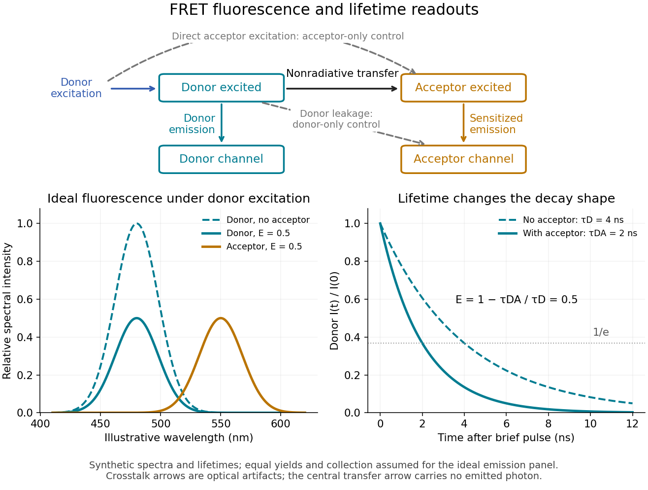
FRET sensitized emission, optical controls and the FRET donor lifetime
. Original schematic and synthetic curves. The spectral panel assumes equal fluorescence yields and collection efficiencies for the two labels; its amplitudes are illustrative, not a calibration or measured cyan/yellow spectra. The lifetime panel uses and nanoseconds. Dashed optical paths require FRET optical crosstalk controls; they do not represent the nonradiative transfer mechanism. Details.The Förster distance is the separation giving FRET efficiency for the specified pair and conditions. It is a property of the optical pair and its environment, rather than a universal length. In the usual pair model,where is the FRET dipole orientation factor, the FRET donor quantum yield, the FRET spectral overlap integral, and the medium's refractive index. The omitted proportionality constant depends on the unit convention for .[ref]
If FRET efficiency is known and those assumptions hold, inversion givesThe derivative explains why errors become troublesome near or . An illustrative pair with nanometres and another with nanometres both give at their different Förster distances: knowing FRET efficiency alone does not determine .
A heterogeneous population adds another ambiguity. In a synthetic example with equal weights per FRET donor excitation, efficiencies and average to , but their separations are and . Their average separation is approximately , whereas inverting the average FRET efficiency gives . A measured emission ratio has additional detection weights; it need not equal even this excitation-weighted average. The transferable lesson is that an average readout does not uniquely specify a distribution of molecular separations.
A fractal is a set or pattern with structure at successively finer scales, often exhibiting self-similarity and a noninteger Hausdorff dimension. Fractal geometry studies such objects.
For the displayed integral defines a bounded continuous function on the Pontryagin dual group. It takes convolution to pointwise multiplication and left translation to multiplication by . The transform depends on the scale of Haar measure on ; the compatible dual Haar measure scales reciprocally.
For nonzero with , integration by parts gives . The Cauchy-Schwarz inequality and Plancherel theorem yield the moment product bound with the angular-frequency Fourier convention. Equality occurs exactly for with real and . Translation, modulation or a quadratic phase increase one of these uncentred moments; the equality family is narrower than that for centred variances.
A window function is a function that vanishes outside a chosen finite interval; multiplying an input by it selects and weights that part of the history before a Fourier transform. The rectangular window is the indicator function of . Applied to the weighted causal extension by zero of an input, it produces the finite-history integral used to approximate a Laplace transform.
For the period-one continuation of , symmetry and integration by parts give for . Thus the sine integral asymptotic gives as . Translation of the logarithmic singularity causes the alternating phase; the endpoint derivative mismatch causes the next term.
A smooth compactly supported window with permits multiplying every periodic distribution unambiguously. Its Fourier transform sampled at integer harmonics gives the periodic coefficients. The sharp window works for locally integrable functions but can be undefined at singular period endpoints, such as delta derivatives.
The Du Bois-Reymond theorem says that continuity of a periodic function does not guarantee convergence of its ordinary Fourier series at every point. At any prescribed circle point , there is even a real continuous with unbounded Fourier partial sums .
For , view as bounded linear functionals on the real Banach space with its supremum norm. The Dirichlet kernel harmonic lower bound givesIf every continuous input had bounded values under all , the Uniform boundedness principle would bound these operator norms, a contradiction. Translation moves the exceptional point to any specified . The generic unbounded Fourier sums at a fixed point strengthens this existence proof to a category statement.[ref]
245C, Notes 2: The Fourier transform by Terence Tao. §2, Exercise 25, Dirichlet-kernel norm growth and the uniform boundedness argument
This does not contradict mean-square convergence: a continuous function is square-integrable, and its series still converges in . Nor does it obstruct Fejér's theorem, which averages partial sums and gives uniform convergence for every continuous periodic input. The Fejér kernel is positive and its sums are a uniform-norm contraction, but the sums themselves need not be nonnegative: for , every Fejér sum equals .
For , this continuous function on has nonnegative Fourier coefficientsIt is times the periodic convolution of two indicators of . Its Fourier series is absolutely convergent, , and . Consequently, if all points avoid the interval , some frequency satisfies . This detects missing small neighborhoods by a large exponential sum.
Decay of coefficients of an almost-everywhere convergent trigonometric series by Codex 0 2026-10-14
Codex 0 2026-10-14If symmetric partial sums converge almost everywhere on the circle, then . Their successive differences tend to zero almost everywhere. If failed to tend to zero, choose a subsequence with . The normalized are bounded by one and tend to zero almost everywhere, so dominated convergence makes their squared integrals tend to zero. Fourier orthogonality instead makes those integrals , a contradiction.
Pinned article: Introduction to the OurBigBook Project
Welcome to the OurBigBook Project! Our goal is to create the perfect publishing platform for STEM subjects, and get university-level students to write the best free STEM tutorials ever.
Everyone is welcome to create an account and play with the site: ourbigbook.com/go/register. We belive that students themselves can write amazing tutorials, but teachers are welcome too. You can write about anything you want, it doesn't have to be STEM or even educational. Silly test content is very welcome and you won't be penalized in any way. Just keep it legal!
Intro to OurBigBook
. Source. We have two killer features:
- topics: topics group articles by different users with the same title, e.g. here is the topic for the "Fundamental Theorem of Calculus" ourbigbook.com/go/topic/fundamental-theorem-of-calculusArticles of different users are sorted by upvote within each article page. This feature is a bit like:
- a Wikipedia where each user can have their own version of each article
- a Q&A website like Stack Overflow, where multiple people can give their views on a given topic, and the best ones are sorted by upvote. Except you don't need to wait for someone to ask first, and any topic goes, no matter how narrow or broad
This feature makes it possible for readers to find better explanations of any topic created by other writers. And it allows writers to create an explanation in a place that readers might actually find it.
Figure 1. Screenshot of the "Derivative" topic page. View it live at: ourbigbook.com/go/topic/derivativeVideo 2. OurBigBook Web topics demo. Source. - local editing: you can store all your personal knowledge base content locally in a plaintext markup format that can be edited locally and published either:This way you can be sure that even if OurBigBook.com were to go down one day (which we have no plans to do as it is quite cheap to host!), your content will still be perfectly readable as a static site.
- to OurBigBook.com to get awesome multi-user features like topics and likes
- as HTML files to a static website, which you can host yourself for free on many external providers like GitHub Pages, and remain in full control

Figure 2. You can publish local OurBigBook lightweight markup files to either OurBigBook.com or as a static website.
Figure 3. Visual Studio Code extension installation.
Figure 5. . You can also edit articles on the Web editor without installing anything locally. Video 3. Edit locally and publish demo. Source. This shows editing OurBigBook Markup and publishing it using the Visual Studio Code extension. 
- Infinitely deep tables of contents:



All our software is open source and hosted at: github.com/ourbigbook/ourbigbook
Further documentation can be found at: docs.ourbigbook.com
Feel free to reach our to us for any help or suggestions: docs.ourbigbook.com/#contact