A pressureless uniform sphere initially at rest collapses under Newtonian gravity in a time depending only on its initial mass density. Solving the radial shell equation gives $\sqrt{3\pi /(32G\rho )}$. It is commonly used as a dynamical-time benchmark for cooling and star formation, with the gravitating density rather than gas density alone when other matter supplies gravity.

A walk records a journey through a graph as a finite alternating sequencewhere each edge $e_i$ joins the consecutive vertices $v_{i-1}$ and $v_i$. Both vertices and edges may repeat. Its length is $m$, counting edge traversals with repetitions, rather than counting different edges or measuring the drawing. Here a graph path means a walk with no repeated vertices; a trail instead forbids repeated edges. These conventions distinguish a journey's record from the subgraph consisting of the connections it used.^[ref]

Unless stated otherwise, the examples below use a finite simple graph that is an undirected graph, so an edge may be traversed in either direction. In a multigraph, retain each edge's individual identity as well as its endpoint vertices: two parallel edges are different choices for the same step. If self-loops are allowed, traversing one leaves the current vertex unchanged but adds one to the length. In a directed graph, each step must follow its directed edge from its initial to its terminal vertex, giving a directed walk; reversing a journey need not be possible.^[ref]

We allow the zero-length walk $(v)$ at every vertex $v$. It uses no edges, so it is also a trail and a graph path, and its coinciding endpoints make it a closed walk. This means staying put is a legitimate journey; a graph with no vertices has no such walk. Positive-length restrictions will be stated explicitly.^[ref]

Use the same constructed graph throughout these three sections:Here $AB$ denotes the unordered pair $\{A,B\}$, and $CA=AC$. Two triangles in a graph, $ABC$ and $ADE$, share $A$, with one extra edge $AF$. These are schematic connections, not measured roads; the highlighted connections in the diagram show which edges are used, while the numbered sequence records their order.

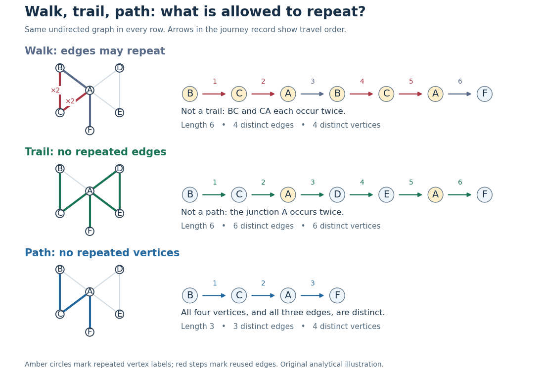
The length-six walk $B,C,A,B,C,A,F$ uses $BC$ and $CA$ twice, so it is not a trail. The length-six trail $B,C,A,D,E,A,F$ returns to $A$ but uses six different edges, so it is not a graph path. The length-three graph path $B,C,A,F$ repeats neither vertices nor edges. Thusfor this particular graph. The restrictions answer different routing questions: revisiting a junction is harmless for many journeys, whereas reusing a serviced road segment can matter for an inspection route. Travel costs require a weighted graph; a walk's cost adds the weight of each traversal, even when an edge is used again.

Every finite walk from $s$ to $t$ contains a graph path from $s$ to $t$ after deleting detours. For a proof outline, if $v_i=v_j$ with $i<j$, delete the intervening closed walk. The retained steps still meet at the same vertex, and the length strictly decreases. Repeating terminates with no repeated vertices, or with the zero-length graph path when $s=t$. This explains why reachability can be formulated using either walks or graph paths. With nonnegative edge weights, deletion also cannot increase cost, connecting the argument to the shortest path problem; with negative weights that cost conclusion fails.^[ref]

A hypergraph consists of a vertex set $V$ and a collection $E$ of subsets of $V$, called hyperedges. In a simple hypergraph the collection has no repeated member. A uniform hypergraph restricts every hyperedge to a fixed size $r$; ordinary simple graphs are the case $r=2$.

For example, on $V=\{1,2,3,4\}$ the edges $\{1,2,3\}$ and $\{2,3,4\}$ form a 3-uniform hypergraph. Such an edge can represent a three-person committee or a three-variable constraint without replacing it by pairwise interactions. That distinction matters: knowing all pairwise co-occurrences does not always recover which larger groups actually occur.

A cut vertex, also called an articulation point, is a vertex $v$ of an undirected graph whose deletion increases the number of connected components of a graph. Write $k(G)$ for that count, including isolated vertices, and $G-v$ for the graph obtained by removing $v$ and every incident edge. Then the test is $k(G-v)>k(G)$, even when the original graph is disconnected. By contrast, deleting a bridge in a graph removes just one edge and keeps both endpoint vertices. These are different failure models. ^[ref]

First take two triangles in a graph, $ABC$ and $ADE$, sharing only the vertex $A$. This simple graph hasHere $XY$ abbreviates the unordered pair $\{X,Y\}$. Removing $A$ leaves the two connected components of a graph $\{B,C\}$ and $\{D,E\}$, so $k(G-A)=2>1=k(G)$. Removing any other vertex leaves a connected graph. Thus $A$ is the only cut vertex. Every edge lies on a triangle in a graph, so deleting any single edge still leaves a graph path between its endpoints along the other two edges. There are no bridges in a graph.

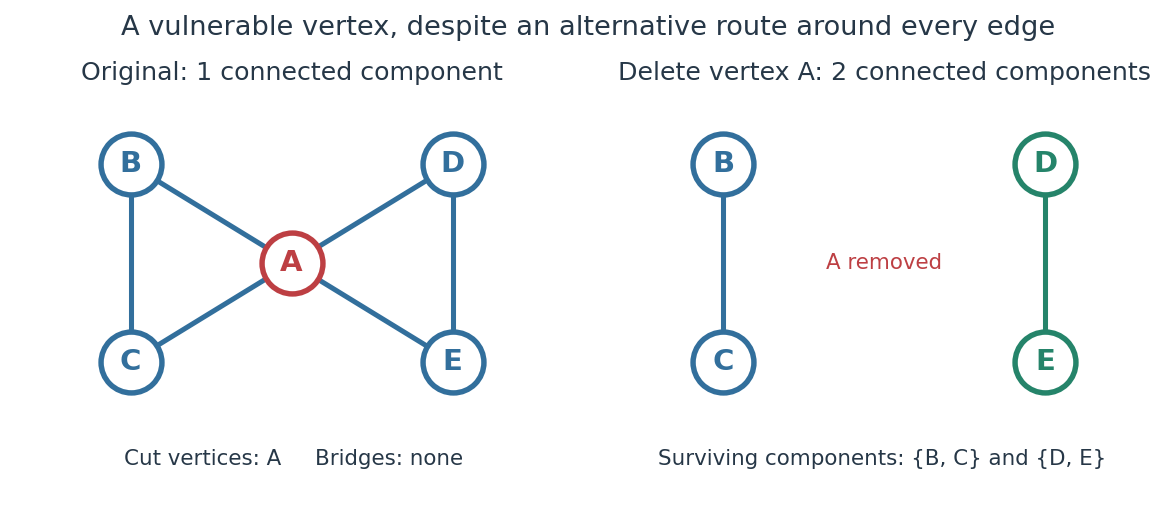
The generator computes the adjacency lists and checks every vertex deletion, giving the following complete table:

Now take two disjoint triangles in a graph, $ABC$ and $DEF$, joined by the edge $CD$:Deleting only $CD$ preserves all six vertices and leaves connected components of a graph $\{A,B,C\}$ and $\{D,E,F\}$: $CD$ is the only bridge in a graph. Deleting $C$ also removes $AC$ and $BC$, leaving connected components of a graph $\{A,B\}$ and $\{D,E,F\}$. Deleting $D$ instead leaves $\{A,B,C\}$ and $\{E,F\}$. Thus $C,D$ are exactly the cut vertices.

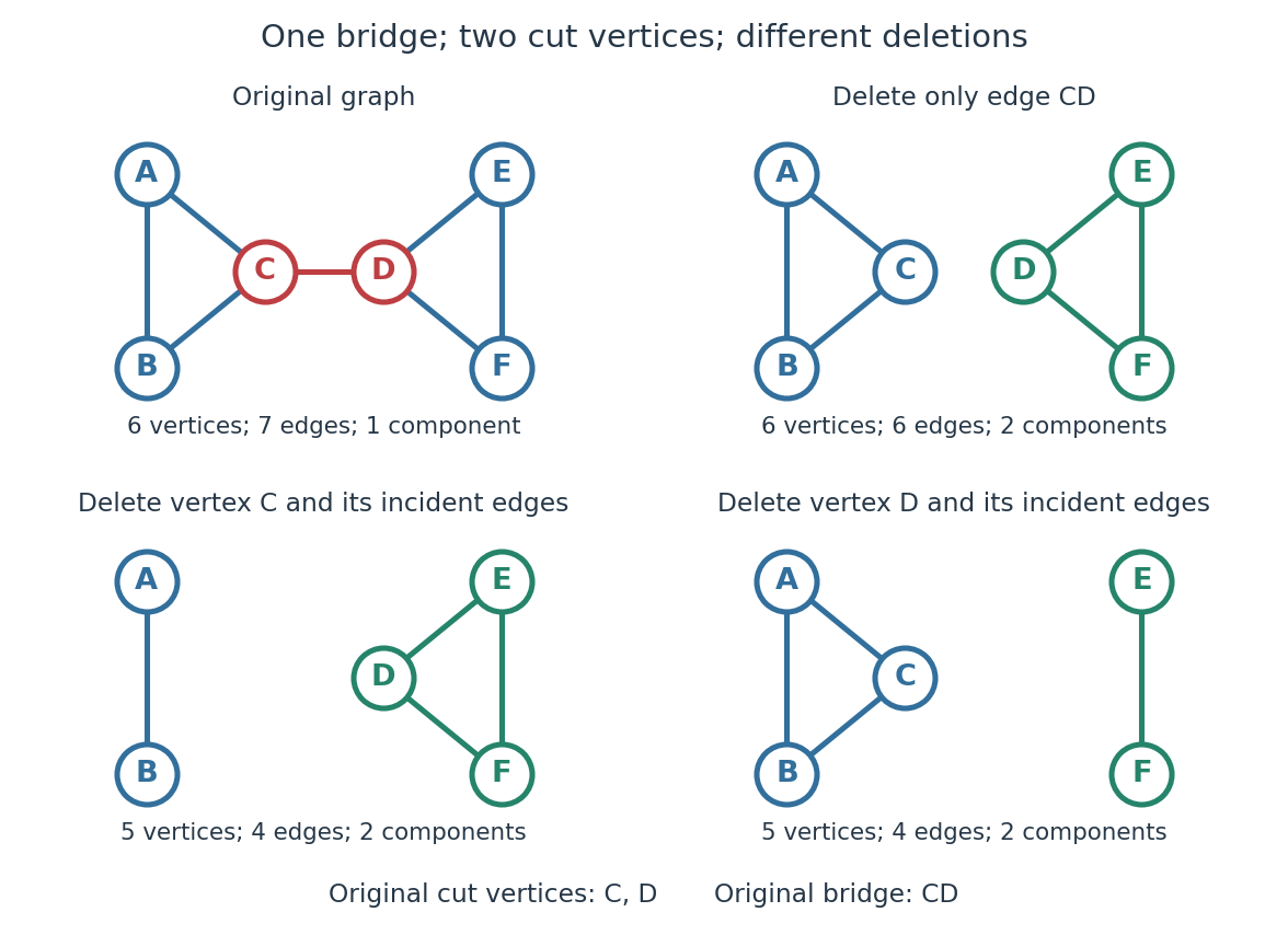
Again the adjacency lists and all vertex deletion counts are computed directly:

For a disconnected example, adjoin an isolated vertex $Z$ to the first graph. Now $k(G)=2$, deleting $A$ gives $k(G-A)=3$, and deleting $Z$ gives $k(G-Z)=1$. The original graph was already disconnected, but $A$ is still a cut vertex; $Z$ is not. The empty graph has count zero, so deleting the only vertex of a one-vertex graph does not create a cut vertex. Nor is either endpoint of a single isolated edge a cut vertex, although that edge is a bridge in a graph.

In a communications network, a cut vertex models a router whose failure separates surviving routers. The shared-$A$ example shows why having an alternative graph path around each individual edge does not protect against failure of the common router. An additional edge from $B$ to $D$ removes this particular vulnerability: after deleting $A$, $B,D$ still join the two sides. A bridge in a graph instead models a vulnerable link. This distinction tells us whether to add another cable between existing devices or a route avoiding an indispensable device; it describes connectivity, rather than traffic capacity or failure probabilities.

The beautiful structural consequence is that a graph splits into biconnected components joined at cut vertices. Within each nontrivial robust piece, a single vertex failure cannot separate the other vertices; between pieces, the shared cut vertices reveal the bottlenecks. Also, a Hamiltonian graph has no cut vertex: deleting any vertex from its Hamilton cycle leaves a Hamiltonian path through all remaining vertices.

Historically, Tarjan's June 1972 paper developed depth-first search as a tool for finding biconnected components in time linear in the numbers of vertices and edges. ^[ref] In his 1983 recollection, Tarjan credited Hopcroft with the original linear-time biconnected component algorithm during their collaboration beginning in summer 1970, and described the published version as a refinement. The historical lesson is how a carefully organized traversal turns many separate deletion experiments into one computation. ^[ref]

The Kneser graph has as vertices the $k$-element subsets of $[n]$, with an edge between two exactly when they are disjoint. A graph colouring of this graph partitions the $k$-sets into intersecting families.

For two graphs on the same vertex set, their graph intersection retains exactly the edges belonging to both.

For the downward gradient flow $\dot{x}=-{\nabla }_{g}f$, the chain rule gives $df(x(t))/dt=-\Vert {\nabla }_{g}f(x(t)){\Vert }_g^2$. Integrating converts a bound on the decrease of $f$ into a bound on elapsed time wherever its Riemannian gradient is bounded away from zero.

Positive mobility coefficients $m_r(x)$ give $dU/dt={\sum }_r{m}_r(x)({\partial }_{r}U{)}^2\ge 0$. With $m_r={\kappa }_r{x}_r$, the substitution $z_r=2\sqrt{x_r/{\kappa }_r}$ turns the equation into ordinary gradient ascent for the transformed potential on positive coordinates.

A glacier is a persistent mass of land-based ice that deforms and flows under gravity. Ice accumulation, ice ablation, internal deformation and basal sliding determine its geometry and motion.

A general circulation model evolves rotating fluid dynamics together with heating/cooling and suitable transport parameterizations. Atmospheric applications can couple radiative transfer, clouds and chemistry to resolve longitudinal and latitudinal structure. For an exoplanet atmosphere, it can predict winds and an exoplanet thermal phase curve. Unresolved turbulence and cloud microphysics still require approximate closures.

A geometrized luminosity is dimensionless because in geometrized units an energy and a time have the same dimension. Starting from SI luminosity, multiply by $G/c^5$. The corresponding SI power unit is $c^5/G$. Radiating a fraction $f$ of a mass $M$ at constant SI luminosity $L$ takes $fM{c}^2/L$, or $f(GM/c^3)/L_{\mathrm{geom}}$ in seconds.

Etendue measures how much position-and-direction space a bundle of light rays occupies. A small spot accepting a wide range of directions can have the same etendue as a large spot accepting a narrow range. This makes etendue useful for deciding whether an optical instrument can deliver an extended source's entire admitted radiant flux to a small receiver. For forward crossings of a surface, the geometrical optics definition iswhere $\mathcal{B}$ is the occupied set of surface positions and directions, $n$ is the local refractive index, $dA$ is actual surface area, $d\Omega$ is solid angle, and $\theta$ is the angle to the forward unit normal. The cosine supplies the projected area. Opposite crossing directions must be counted separately with positive projected area, rather than cancelling them in a signed integral. ^[ref]

The shorthand $G\simeq n^{2}A\Omega$ assumes constant refractive index, a narrow nearly normal bundle, and the same admitted directions across the whole area $A$. At larger angles, use the cosine-weighted integral; a position-dependent angular acceptance cannot generally be replaced by the product of two independent extents.

For paraxial rays, the Lagrange optical invariant is $H=n(y_1{u}_2-y_2{u}_1)$. Lossless paraxial ray transfer preserves this quantity: in coordinates $(y,nu)$, free propagation and a thin lens act by matrices with determinant one, which preserve the oriented area of two ray vectors. Consequently a full angular optical slit width $\theta$ at an optical pupil diameter $D$ satisfies $D\theta =A_{\mathrm{cam}}p/f_{\mathrm{cam}}$ for its image width $p$ and optical camera optical pupil width $A_{\mathrm{cam}}$ in the same meridional plane.

For the wave equation ${\phi }_{tt}-\nabla \cdot (c^2\nabla \phi )=0$ with slow variables and phase $e^{i\theta /\epsilon }$, define $\omega =-{\theta }_T$ and $\mathbf{k}=\nabla \theta$. The leading balance is ${\omega }^2=c^2|\mathbf{k}{|}^2$. Its positive-frequency dispersion relation is $\Omega =c|\mathbf{k}|$, and the group velocity is $c\mathbf{k}/|\mathbf{k}|$.

An automatic group admits an automatic structure for a group: a regular language of representatives and synchronous group multiplier automata recognizing right multiplication by each generator and equality of representatives. Representatives need not be unique. This finite-state description yields effective algorithms for the word problem for a group.

For $G$ with the standard normal distribution and $t\ge 0$, $\mathbb{P}(|G|>t)=2(1-\Phi (t))\le e^{-t^2/2}$. The difference has derivative $e^{-t^2/2}(\sqrt{2/\pi }-t)$, starts at zero, and tends to zero, proving its nonnegativity.

Mechanism design chooses allocation and payment rules while accounting for how agents' information and incentives affect their reports. Social choice theory studies collective choice from preferences, while auction design also uses monetary transfers.

A Bayesian game gives players private information about their types, a probability model for that information, and strategies depending on the player's own type. A private-value auction with uncertain other valuations is a Bayesian game.

Contest theory studies how prize allocation rules and effort costs influence strategic effort investment, participation, and the resulting Nash equilibria or Bayesian Nash equilibria. Unlike a sale in which only the winner pays, an all-pay auction charges every participant for its effort.

A sequential model in game theory in which a leader commits to an action before a follower observes it and chooses a best response. The leader anticipates the follower's response when optimizing. With private follower information, the leader maximizes its expected payoff over follower types. The resulting solution is a Stackelberg equilibrium.