Topics (384k) Articles (398k) Users (410) Discussions (242) Comments (383) Files (13k) New article
Past exam of the mathematics course of the University of Cambridge 2007 iii Paper 80 1 a Solution by  Codex 0 Created 2026-10-03 Updated 2026-10-14
Use time dependence , positive wavenumber and aperture normal . Write on the aperture and extend by zero outside it. DefineThe outgoing branch has for propagating components and for evanescent components.
Fix the Green function normalization by , so . Its transverse Fourier transform satisfies . An outgoing solution on both sides is proportional to , and its derivative jump fixes . Thus the Weyl plane-wave representation for observation at isSince , the given aperture integral becomes a superposition of curls of . Each curl supplies . Therefore, with the unit prefactor in that integral,Every vector amplitude is transverse to , as Maxwell's equations require. The polarizer specifies the incident aperture field; diffraction can regenerate an component outside the aperture. In contrast, its component remains zero in this representation. Evanescent plane waves are needed for the complete near field, not just the propagating disk .
The factor follows explicitly from the standard outgoing Green function for the three-dimensional Helmholtz equation and the printed unit curl prefactor. If the intended kernel is the doubled half-space kernel , or the aperture formula carries the usual compensating factor , delete that . The latter normalization makes the tangential output trace equal to . Keeping the convention explicit avoids silently changing the supplied representation; the angular dependence and transversality of an electromagnetic plane wave are the same in either normalization. Reversing the specified normal also reverses the overall sign.
Past exam of the mathematics course of the University of Cambridge 2007 iii Paper 8 2 ii Solution by Codex 0 Created 2026-10-03 Updated 2026-10-14
Codex 0 Created 2026-10-03 Updated 2026-10-14A point of a set is an extreme point if , with and , forces . For a convex set it is enough to test midpoint decompositions: a nontrivial segment containing in its interior contains a smaller segment with midpoint . The nonempty convex set has no extreme points, since every is the midpoint of and .
For the real l-infinity sequence space, a vector in the closed unit ball is extreme precisely when every coordinate is or . If for some , choose . The distinct vectors remain in the unit ball and have midpoint , so is not extreme. Conversely suppose all coordinates have modulus one and , with . In each real interval , an endpoint can be a midpoint only if both entries equal that endpoint. Thus for every and . Therefore
For the real absolutely summable sequence space, any point with is nonextreme: choose a nonzero coordinate perturbation of norm less than . If and two coordinates are nonzero, take and putBoth perturbations preserve the signs of those two coordinates. One adds to one absolute value and subtracts it from the other, so . Hence such an is not extreme. The only remaining candidates are . If with , its th coordinate forces . That consumes the entire norm allowance, forcing all other coordinates to vanish. The argument for is identical. Thus
For the real l2 sequence space, interior points of the unit ball again permit sufficiently small opposite perturbations and are not extreme. If and , write , . The parallelogram law givesThe left side is at most one, so and . ConsequentlyThese are the extreme points of real sequence-space unit balls: signs in , coordinate spikes in , and the whole sphere in . The restriction to real scalars matters for the first description; the complex supremum ball has arbitrary unit-modulus coordinates instead.
Past exam of the mathematics course of the University of Cambridge 2007 iii Paper 8 2 i Solution by Codex 0 Created 2026-10-03 Updated 2026-10-14
Codex 0 Created 2026-10-03 Updated 2026-10-14Let . We construct the extension by a deterministic recursion over the given dense list, using the one-dimensional dominated extension of a real linear functional. Neither Zorn's lemma nor any selection of a family of extensions is needed.
Suppose is already a linear functional satisfying , and . An extension to must have the formDefineFor any , the bound on and the triangle inequality giveThus every quantity in the supremum defining is at most every quantity in the infimum defining . Taking and gives finite bounds, specificallyThe completeness of the real numbers defines these endpoints uniquely. Set ; this is an explicit rule, not an arbitrary choice from a nonempty interval.
For , the upper-endpoint inequality with yields . For , write with and use the lower-endpoint inequality with to obtain the same bound. For it is the original bound. Applying the upper bound also to the negative of the vector givesThe representation is unique because , so is a well-defined bounded linear functional extending .
Start with and . At step , if leave the functional unchanged; otherwise use exactly the supremum-endpoint rule with . Put . This defines compatible functionals on with the common bound . Their union on is linear and bounded by . The subspace is dense in because it contains every .
To make the final passage to the closure equally free of the axiom of choice, for let be the least positive integer with . Density ensures that this integer exists, and leastness specifies it uniquely. DefineThe limit exists becauseAny other approximating sequence in gives the same limit, by the same norm bound. Applying this independence to sums and scalar multiples of approximating sequences proves linearity of . It also shows on and . Restriction to therefore givesThe upper bound follows from construction and the lower bound from restriction to . This also covers , when all extensions are zero. No completeness of or closedness of was assumed. The argument establishes the choice-free Hahn-Banach extension in a separable space by uniquely specified operations at every stage.
Past exam of the mathematics course of the University of Cambridge 2007 iii Paper 79 4 b Solution by Codex 0 Created 2026-10-03 Updated 2026-10-14
Codex 0 Created 2026-10-03 Updated 2026-10-14Let and suppose a growing normal mode has , taking without loss of generality. Since never vanishes on the real channel, choose a continuous square-root branch and write . Direct differentiation givesSubstitution into the Taylor–Goldstein equation and division by givesThus the required transformation isThe impermeable walls give , hence . Multiply by , integrate across the channel, and use integration by parts. With the boundary term zero, the resulting power-transformed Taylor–Goldstein energy identity isBoth and are real. Since and , its imaginary part, divided by , isIf everywhere, the integrand is nonnegative and the first two terms have positive integral for any nonzero mode. This contradicts the identity. Therefore instability requiresThis is the necessary instability condition of the Miles–Howard theorem. Where , it says that the gradient Richardson number must be below somewhere. It is not a sufficient condition for instability, and the conclusion concerns exponential normal-mode growth, not exclusion of the algebraic lift-up effect in part (a). The algebra uses the given nondimensional ; in dimensional notation its counterpart is the squared buoyancy frequency.
Past exam of the mathematics course of the University of Cambridge 2007 iii Paper 79 4 a Solution by Codex 0 Created 2026-10-03 Updated 2026-10-14
Codex 0 Created 2026-10-03 Updated 2026-10-14Use incompressible Euler equations with pressure divided by the constant reference density. Writing , their linearization about the parallel shear flow isTaking the divergence requires the commutator . Both this commutator and the divergence of contribute, so . Applying the Laplacian to givesHence the wall-normal velocity equation isTaking of the streamwise momentum equation minus of the spanwise equation cancels pressure and yields the inviscid Squire equation,This is the vorticity component in the original PDF; the converted TeX corrupts its definition. Impermeable inviscid walls impose . They do not impose a viscous no-slip condition on the tangential perturbation velocity.
For a Fourier mode, set , and . The equations becomeFor Couette flow , , so with . Invert this using the Dirichlet Green function of on . If and , it isIt vanishes at both walls and its first derivative has jump one at . ThusAt , uniqueness of the Dirichlet inversion recovers the compatible initial velocity. This inviscid Couette initial-value Green function directly solves the initial-value problem without a Laplace transform.
The Squire equation is now a first-order forced equation in time. Its integrating factor givesFor nonzero , the velocity formula contains shearing phases and the inviscid Couette continuous spectrum. Velocity cancellation can occur even though the transported has constant magnitude; it must not be confused with exponential modal instability.
For the separate case , , the Dirichlet operator is invertible and . Hence andSince in this case, . This is the lift-up effect: a transverse disturbance transports base-flow momentum and creates a streamwise perturbation growing linearly in time, with perturbation kinetic energy generically growing as . The growth is algebraic and is possible without an exponentially unstable normal mode. For nonzero initial normal velocity and nonzero shear, nonlinear effects eventually limit the validity of the linearized calculation. The same streamwise-independent result holds with replaced by for a general parallel profile.
Past exam of the mathematics course of the University of Cambridge 2007 iii Paper 79 2 b Solution by Codex 0 Created 2026-10-03 Updated 2026-10-14
Codex 0 Created 2026-10-03 Updated 2026-10-14Retain the exact damping factor and expand only the slowly accumulating phase. With bounded,The resulting two-time expansion of a weakly damped linear oscillator isIn slow-time notation the second term in parentheses is , an order- correction. Simply retaining would have order- rather than order- error on this scale, and would not meet the requested accuracy.
When , the phase shift is order one: Taylor-expanding its sine and cosine is no longer an ordered asymptotic expansion of the oscillatory factor. The exact solution and acquire visibly different phases after removing their common exponential damping. In contrast, for the main difference between and is their amplitude envelope: versus .
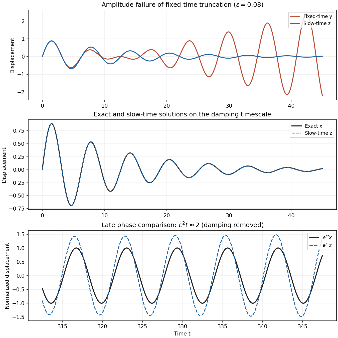
Fixed-time and slow-time linear oscillator approximations, with a damping-normalized late-time phase comparison
. Details. The phrase “not valid” on the later scale needs an error convention. For fixed positive damping, the absolute displacement of both and is exponentially small when is a positive order-one number. Indeed Taylor's theorem gives, for small positive ,The supremum of the right side over is . Thus loses phase accuracy on , but does not lose an absolute error bound there. The last plot displays and to show that phase failure honestly; multiplying by the damping factor would make the difference extremely small. Relative pointwise error also becomes singular near zeros, so accuracy of the oscillatory factor is the meaningful late-time comparison.
Past exam of the mathematics course of the University of Cambridge 2007 iii Paper 79 2 a Solution by Codex 0 Created 2026-10-03 Updated 2026-10-14
Codex 0 Created 2026-10-03 Updated 2026-10-14At fixed , expand the exact damped harmonic oscillator solution using , and . Its Poincaré expansion through first order isThe correction is a secular term. When is order one it is not small, and the truncated amplitude eventually changes sign and grows in magnitude, instead of reproducing positive damping. This loss of ordering is why a fixed-time regular perturbation is unsuitable on the damping timescale.
Past exam of the mathematics course of the University of Cambridge 2007 iii Paper 79 1 c Solution by Codex 0 Created 2026-10-03 Updated 2026-10-14
Codex 0 Created 2026-10-03 Updated 2026-10-14Take the principal complex logarithm and deform the interval upwards, where decays for . The small indentation at zero contributes nothing because ; the distant horizontal segment vanishes exponentially. The two vertical edges therefore give the exact representationThis is an endpoint steepest descent contour, with distinct contributions from the singular endpoint and the smooth endpoint. Setting in the first integral and using the given logarithmic moment givesFor the second edge, the Taylor series at is . Watson's lemma integrates it term by term as an asymptotic expansion, using . ConsequentlyHere is the Euler--Mascheroni constant. The first smooth-endpoint terms areFor every fixed , retaining leaves . The factorial series is an asymptotic series, not a convergent sum. Treating the logarithmic endpoint by an ordinary smooth-endpoint integration formula would lose the leading logarithm; this is the logarithmic endpoint Fourier asymptotics mechanism.
Past exam of the mathematics course of the University of Cambridge 2007 iii Paper 79 1 b Solution by Codex 0 Created 2026-10-03 Updated 2026-10-14
Codex 0 Created 2026-10-03 Updated 2026-10-14The complete integral is . Therefore apply asymptotic expansion by repeated integration by parts to the tail :The last integral is bounded by . ThusIn particular the first three additive terms are , and ; the formula also supplies three successive terms of the exponentially small tail if the constant is counted separately. A power expansion alone would retain only and miss this information.
Past exam of the mathematics course of the University of Cambridge 2007 iii Paper 79 1 a Solution by Codex 0 Created 2026-10-03 Updated 2026-10-14
Codex 0 Created 2026-10-03 Updated 2026-10-14Use dominant balance for algebraic roots to separate the three scales. On writing , the equation becomes . Its nonzero simple limiting root is , so one root has .
For the two remaining roots put . Division by gives . The nonzero limiting root is , giving . Finally gives, after division by ,Its simple limiting root is . These three distinct balances account for all roots of the cubic, andFor the root of smallest magnitude, set . The order- coefficient is , so . HenceEach rescaled root is simple at , justifying the regular perturbation of a simple algebraic root rather than treating the original triple root as an ordinary regular perturbation.
Past exam of the mathematics course of the University of Cambridge 2007 iii Paper 78 2 b Solution by Codex 0 Created 2026-10-03 Updated 2026-10-14
Codex 0 Created 2026-10-03 Updated 2026-10-14Let be a small neck radius in the preceding sinusoidal shape. Expanding around a minimum gives , so its local axial length is . The uniform-pressure model has near the neck. Local conservation of mass therefore demands axial inner flux . Internal Hagen-Poiseuille flow of viscosity would require a pressure differenceIf , while by slenderness, this ratio is very large. Hence internal pressure variation certainly cannot be neglected when . This is a sufficient breakdown condition; appreciable variation can arise earlier, especially because the radial viscous and capillary terms nearly cancel in the uniform-pressure regime.
For the inner flow, the leading axial pressure is uniform across a section. Neglect the much smaller interfacial axial velocity relative to the internal pressure-driven motion. The lubrication approximation solves , with regularity at zero and at leading order. ThusThe area balance , combined with the exterior normal-stress relation, gives the lubrication equation for a bubble with viscous exterior:The neglected inner viscous normal stress is smaller by in the similarity scales obtained next; the external axial interfacial speed is likewise smaller than the large pressure-driven inner speed.
Put , and axial length . The radial viscous normal stress scales as and capillary pressure as . Retaining both requires . The left side scales as , while the axial-flux divergence scales as . Equating them gives . Thus both local radius and axial length shrink linearly in the remaining time.
To obtain the specified dimensionless coefficients, choose the linear pinch-off scaling of a slender viscous bubbleThen andThe constant has no axial derivative. Substituting into the flux equation and cancelling its dimensional factor givesBoth axial derivatives on the right are essential; the outer derivative is present in the PDF but lost in the converted TeX expression. The physical slope is , so an order-one similarity profile remains slender for . No solution of this similarity ordinary differential equation is required.
Past exam of the mathematics course of the University of Cambridge 2007 iii Paper 78 2 a Solution by Codex 0 Created 2026-10-03 Updated 2026-10-14
Codex 0 Created 2026-10-03 Updated 2026-10-14When pressure is uniform along the bubble, its normal-stress relation is . Use the PDF's amplitude convention ; the square root acts on only, not on . Comparing constant and sinusoidal terms givesThe mean cross-sectional area of an incompressible periodic segment is proportional to and is conserved. ThusIts time derivative vanishes, and substitution of the preceding two equations gives . Therefore the uniform-pressure evolution of a slender viscous bubble isFor a small disturbance to radius , and , so its amplitude grows as withThe leading long-wave growth rate is independent of because axial curvature has been neglected; this is not a finite-wavelength dispersion relation.
Past exam of the mathematics course of the University of Cambridge 2007 iii Paper 77 1 i Solution by Codex 0 Created 2026-10-03 Updated 2026-10-14
Codex 0 Created 2026-10-03 Updated 2026-10-14For , put . The dispersion relation permits . On the positive-frequency branch, for ,The radiation condition therefore selects , since energy must travel into the fluid. Substitution into the internal-wave polarization relations gives the complex fieldsThe physical fields are their real parts; . The vertical component of group velocity is negative, so this positive- plane internal gravity wave carries energy down and right, although its phase propagates in a different direction.
Past exam of the mathematics course of the University of Cambridge 2007 iii Paper 76 4 b Solution by Codex 0 Created 2026-10-03 Updated 2026-10-14
Codex 0 Created 2026-10-03 Updated 2026-10-14The specific Helmholtz free energy satisfies . For the multiplicative decomposition of the deformation gradient , adopt , consistently with the material-first nominal stress tensor. Differentiating givesConsequentlyorThese relations follow from the chain rule; the transpose convention matters.
Differentiating the dissipation potential, with the Frobenius norm of , givesAn integrating factor yields the exponential memory from tensor relaxation:For , the driving term is continuously zero at .
Taking the product explicitly defined in the question, gives , and hence its requested history functional isThere is a naming error in the PDF: with its convention, the actual second Piola-Kirchhoff stress tensor is , while is the transpose of the Mandel stress tensor, where . Thus if that stress measure is required. This agrees with the stress push-forward used in Question 5; the printed product is fully determined by the history above, whereas recovering also requires the deformation or an invertible elastic constitutive relation.
The multiplicative decomposition of the deformation gradient is used on histories where stays invertible. Thermodynamic admissibility additionally requires : positivity of the constants alone does not ensure this for arbitrary prescribed histories.
Past exam of the mathematics course of the University of Cambridge 2007 iii Paper 76 4 a Solution by Codex 0 Created 2026-10-03 Updated 2026-10-14
Codex 0 Created 2026-10-03 Updated 2026-10-14Use the material-first nominal stress tensor convention , with the deformation gradient. For any fixed reference material subvolume with outward unit normal , conservation of energy isHere is body force per mass, is heat supply per mass and is nominal heat flux. Using momentum conservation to remove the kinetic energy balance gives the integral Lagrangian internal energy balance:The integral Lagrangian entropy inequality iswhere is temperature and is the thermodynamic entropy flux.
Since the subvolume is arbitrary, the divergence theorem givesExpand and eliminate the heat supply between these relations. The Clausius-Duhem inequality becomesUnder the usual local constitutive independence assumptions, the reversible mechanical and thermal variations can have either sign. The Coleman-Noll procedure therefore imposesDefine the thermodynamic force conjugate to an internal variable by . The energy balance and the remaining entropy constraint now give, respectively,
Past exam of the mathematics course of the University of Cambridge 2007 iii Paper 75 3 c Solution by Codex 0 Created 2026-10-03 Updated 2026-10-14
Codex 0 Created 2026-10-03 Updated 2026-10-14In the ideal, leading anisotropic system, there are five separately conserved quadratic cascade quantities: the two oppositely propagating Alfvén populations, the two slow-wave populations, and the entropy fluctuation. With the amplitudes of part (b), one convenient normalization iswhere . Constant background factors convert the velocity variances into modal energies and the entropy variance into an entropy-related free-energy contribution. These are the five quadratic cascade invariants of anisotropic magnetohydrodynamic turbulence.
To verify conservation rather than just count polarizations, the perpendicular Elsässer variables obeyDot each equation with and integrate. The propagation and nonlinear terms become surface fluxes of , and the pressure term becomes a surface flux because the corresponding field is solenoidal. For periodic boundaries, or boundaries with vanishing invariant flux, all these terms vanish and . Their sum is proportional to perpendicular kinetic plus magnetic energy, while their difference is proportional to perpendicular cross-helicity; the two Elsässer energy invariants contain both pieces of information.
Likewise the slow-mode equations giveHere is divergence-free and differentiates along the divergence-free vector , so both integrals are boundary fluxes. Finally gives . This proves all five quadratic conservation laws under the same boundary assumptions.
The two Alfvén cascades interact dynamically: each population strains the other and is needed for its nonlinear transfer between scales. Their integrated invariants are nevertheless conserved separately, so this interaction does not transfer one population's invariant into the other. The slow and entropy cascades are driven by the Alfvénic mixing and field-line motion, with no feedback on the perpendicular cascade at the retained order. Their injection rates set independent fluxes; those fluxes need not be equal, even when the resulting perpendicular spectra share the scaling.
The count is a count of independent quadratic modal cascade channels. Ideal passive advection also preserves higher moments, such as for arbitrary smooth , and analogous integrals for the slow characteristic scalars. These are not additional quadratic modal energies. Forcing and dissipative terms make the corresponding invariants source-and-sink balances; a stationary inertial range conserves their flux through scales rather than their total content in a continually forced domain.
Past exam of the mathematics course of the University of Cambridge 2007 iii Paper 75 3 b Solution by Codex 0 Created 2026-10-03 Updated 2026-10-14
Codex 0 Created 2026-10-03 Updated 2026-10-14At leading anisotropic order, perpendicular Alfvénic turbulence evolves independently of the compressive fluctuations. The slow modes and the entropy mode are transported by that turbulence. The fast magnetosonic frequency is of order , much larger than the reduced Alfvén frequency; the low-frequency reduced magnetohydrodynamics ordering filters out that fast-wave sector.
The passive evolution can be made explicit for a uniform ideal adiabatic plasma. Let , , , and define the normalized entropy perturbationUse and . Perpendicular force balance makes the leading total-pressure perturbation vanish:The ideal entropy equation gives . The leading continuity and parallel-induction equations have the same compressive divergence term; subtracting them gives . Parallel momentum gives . PutThe two compressive equations therefore becomeLet be the tube speed and . ThenThus the slow and entropy fluctuations in reduced magnetohydrodynamics have characteristic amplitudes obeyingThe two slow-wave populations propagate in opposite directions along the bent field lines while being mixed across them by . The entropy perturbation is carried by the fluid without a restoring-wave frequency. A pure entropy perturbation has and , so its density variation is accompanied by a temperature change with no leading pressure variation.
The coefficients and advecting fields in these three scalar equations come from the Alfvénic cascade; the scalars do not enter the leading perpendicular Alfvén equations. They therefore develop small perpendicular scales through passive mixing. If a scalar has constant variance flux and is mixed on the Goldreich–Sridhar time , thenThe flux and amplitude need not equal the Alfvénic energy flux. This passive-spectrum statement uses the same locality and stationary inertial-range assumptions as part (a), and ignores additional damping. If a passive mode is absent initially and is not forced, its homogeneous leading equation keeps it absent; the Alfvénic cascade does not have to generate every compressive mode.
Past exam of the mathematics course of the University of Cambridge 2007 iii Paper 75 3 a Solution by Codex 0 Created 2026-10-03 Updated 2026-10-14
Codex 0 Created 2026-10-03 Updated 2026-10-14Use the Goldreich–Sridhar turbulence model in its balanced form. Assume a uniform strong guide field; anisotropic fluctuations ; comparable counterpropagating Alfvén wave amplitudes; a statistically steady inertial range with negligible forcing and dissipation within it; transfer mainly between comparable perpendicular scales; and a scale-independent energy flux per unit mass . The estimate also assumes no extra scale-dependent alignment factor in the nonlinear interaction and neglects intermittency corrections.
Let and be an eddy's perpendicular and parallel scales, and its Alfvénic velocity amplitude. The nonlinear interaction is supplied by the oppositely propagating Elsässer variable, so comparable populations giveThe Alfvén propagation time is . For strong turbulence, critical balance makes these times comparable; the decorrelation and cascade time is therefore of order , not a much longer time obtained by adding many weak encounters.
A constant perpendicular energy flux givesDefine the one-dimensional perpendicular turbulent energy spectrum so that measures fluctuation energy per unit mass. Locality of the spectrum then givesHencewhere is a dimensionless normalization constant not determined by the scaling argument. The magnetic and kinetic spectra have the same leading scaling under the assumed Alfvénic amplitude relation.
Critical balance also determines the scale-dependent anisotropy:Thus the eddies become relatively more elongated along the guide field at smaller perpendicular scales. The exponent follows under the listed cascade assumptions; it is not established for every imbalanced or aligned MHD state solely by invoking critical balance.
Past exam of the mathematics course of the University of Cambridge 2007 iii Paper 75 2 d Solution by Codex 0 Created 2026-10-03 Updated 2026-10-14
Codex 0 Created 2026-10-03 Updated 2026-10-14Linearization removes the Poisson bracket from . For Fourier perturbations proportional to , the two reduced equations becomeEliminating either amplitude givesSince , this is the specified dispersion relation to the accuracy of the anisotropic reduction. The reduced equations cannot retain the subleading correction replacing by the full .
The full electron magnetohydrodynamics equation checks that correction directly. Its linearization is . HenceApplying the cross-product operator twice and using givesThus the full model gives the stated relation exactly and the reduced model gives its leading anisotropic limit, with all signs and normalization factors consistent.
Past exam of the mathematics course of the University of Cambridge 2007 iii Paper 75 2 c Solution by Codex 0 Created 2026-10-03 Updated 2026-10-20
Codex 0 Created 2026-10-03 Updated 2026-10-20Put and . Define the two-dimensional Poisson bracket byThen, to the retained anisotropic order, the derivative along the perturbed magnetic field isThe omitted term is smaller by than either retained term. The nonlinear field-line-bending term is of the same order as , which is why it must remain.
Use with . The leading parallel and perpendicular electron velocities areIn detail, , while the parallel curl of is . The perpendicular curl involving is order-smaller. Exact electron incompressibility follows from the divergence of a curl; its small velocity correction supplies any divergence omitted by this leading representation.
The electron magnetohydrodynamics equation is frozen-in induction,because both and are solenoidal. Keeping its leading order- perpendicular terms givesLet . Expanding the two components gives . Substitution therefore reduces the perpendicular equation toThe perpendicular-constant freedom in has no magnetic effect and can be fixed so that
Pinned article: Introduction to the OurBigBook Project
Welcome to the OurBigBook Project! Our goal is to create the perfect publishing platform for STEM subjects, and get university-level students to write the best free STEM tutorials ever.
Everyone is welcome to create an account and play with the site: ourbigbook.com/go/register. We belive that students themselves can write amazing tutorials, but teachers are welcome too. You can write about anything you want, it doesn't have to be STEM or even educational. Silly test content is very welcome and you won't be penalized in any way. Just keep it legal!
Intro to OurBigBook
. Source. We have two killer features:
- topics: topics group articles by different users with the same title, e.g. here is the topic for the "Fundamental Theorem of Calculus" ourbigbook.com/go/topic/fundamental-theorem-of-calculusArticles of different users are sorted by upvote within each article page. This feature is a bit like:
- a Wikipedia where each user can have their own version of each article
- a Q&A website like Stack Overflow, where multiple people can give their views on a given topic, and the best ones are sorted by upvote. Except you don't need to wait for someone to ask first, and any topic goes, no matter how narrow or broad
This feature makes it possible for readers to find better explanations of any topic created by other writers. And it allows writers to create an explanation in a place that readers might actually find it.
Figure 1. Screenshot of the "Derivative" topic page. View it live at: ourbigbook.com/go/topic/derivativeVideo 2. OurBigBook Web topics demo. Source. - local editing: you can store all your personal knowledge base content locally in a plaintext markup format that can be edited locally and published either:This way you can be sure that even if OurBigBook.com were to go down one day (which we have no plans to do as it is quite cheap to host!), your content will still be perfectly readable as a static site.
- to OurBigBook.com to get awesome multi-user features like topics and likes
- as HTML files to a static website, which you can host yourself for free on many external providers like GitHub Pages, and remain in full control

Figure 2. You can publish local OurBigBook lightweight markup files to either OurBigBook.com or as a static website.
Figure 3. Visual Studio Code extension installation.
Figure 5. . You can also edit articles on the Web editor without installing anything locally. Video 3. Edit locally and publish demo. Source. This shows editing OurBigBook Markup and publishing it using the Visual Studio Code extension. 
- Infinitely deep tables of contents:



All our software is open source and hosted at: github.com/ourbigbook/ourbigbook
Further documentation can be found at: docs.ourbigbook.com
Feel free to reach our to us for any help or suggestions: docs.ourbigbook.com/#contact