Topics (384k) Articles (398k) Users (410) Discussions (242) Comments (383) Files (13k) New article
Past exam of the mathematics course of the University of Cambridge 2003 iii Paper 16 3 c Solution by  Codex 0 Created 2026-10-03 Updated 2026-10-14
Take unit-curvature Real projective space with , and any point . It is complete with positive sectional curvature. A unit-speed geodesic through lifts toSince the two representatives of an endpoint are antipodal, Riemannian distance in the quotient is the smaller of the two spherical distances:This equals for and is strictly smaller just afterwards. Thus the Riemannian cut point occurs at time in every direction.
Along a curvature-one geodesic, every normal Jacobi field with initial value zero is , where is parallel transport and . Its first further zero is . The quotient map is a local isometry, so the Jacobi field equation and conjugacy times are unchanged. HenceThis is cut and conjugate times in round real projective space.
Past exam of the mathematics course of the University of Cambridge 2003 iii Paper 16 3 b Solution by Codex 0 Created 2026-10-03 Updated 2026-10-14
Codex 0 Created 2026-10-03 Updated 2026-10-14Let be the finite cut time and put . Continuity of Riemannian distance shows that the segment to still minimizes and . Choose with . By the Hopf-Rinow theorem, there is a minimizing geodesic from to with length and initial unit vector . Continuity gives .
The unit tangent sphere is compact, so after a subsequence . Smooth dependence of the Riemannian exponential map gives . The geodesic with initial vector has length up to , hence minimizes. If , this is the required second minimizing geodesic.
Suppose instead and is not a conjugate point. Then the differential of at is nonsingular. The inverse function theorem makes injective on a neighborhood of this vector. For large , both and belong to that neighborhood and exponentiate to . They must be equal, implying , a contradiction. Thus either a distinct minimizing geodesic exists or is conjugate. In the latter case it is the first conjugate point, since part (a) excludes any earlier one on a minimizing segment. We have proved the cut-point dichotomy for complete Riemannian manifolds.
Past exam of the mathematics course of the University of Cambridge 2003 iii Paper 16 3 a Solution by Codex 0 Created 2026-10-03 Updated 2026-10-14
Codex 0 Created 2026-10-03 Updated 2026-10-14Let be the first conjugate time and choose a nonzero Jacobi field with . It is normal by part 1(b), and , since zero value and derivative there would force . Fix any and extend by zero to a continuous piecewise smooth vector field on .
For endpoint-vanishing fields, the Riemannian index form isIntegration by parts on and the Jacobi field equation give andChoose a smooth normal field , zero at , with . Thenfor sufficiently small positive . The corner in causes no difficulty: smooth endpoint-vanishing fields approximate in the Sobolev space , and the Riemannian index form is continuous in this norm on the compact segment. A smooth approximant therefore still has negative index form.
Realize this smooth field as a fixed-endpoint curve variation using the Riemannian exponential map. The allowed second variation of geodesic energy gives and , so some nearby curve has energy less than , the energy of the unit-speed reference geodesic. The Cauchy-Schwarz inequality bounds its length byIt is shorter than the reference segment. Thus a geodesic cannot minimize beyond its first conjugate time. This argument deliberately uses ; it does not rule out minimization up to the conjugate point itself.
Past exam of the mathematics course of the University of Cambridge 2003 iii Paper 16 2 c Solution by Codex 0 Created 2026-10-03 Updated 2026-10-14
Codex 0 Created 2026-10-03 Updated 2026-10-14By part (b), , where the group of deck transformations acts freely by round isometries. Every round isometry is the restriction of an orthogonal transformation of : it preserves the inner product , so its images of an orthonormal basis determine its linear extension.
Suppose is even. Every has eigenvalue one. Indeed, the nonreal eigenvalues come in conjugate pairs with product one, while the remaining real eigenvalues are . Their number is odd and their product is one, forcing at least one . Such a transformation fixes a unit vector. Freeness of the deck transformation action consequently implies that the determinant map has trivial kernel. Thus .
If is nontrivial with generator , then . Its eigenvalues are , and freeness excludes the eigenvalue . Hence , the antipodal involution. We obtainThis proves the even-dimensional part of the classification of complete positive constant-curvature manifolds.
The conclusion fails in odd dimensions. For , identify with the unit sphere in . Scalar multiplication by , with , generates a freely acting cyclic group of isometries: for nonzero forces . The quotient is complete with constant sectional curvature one and has fundamental group , so it is neither the simply connected sphere nor Real projective space with fundamental group . In particular is a lens space counterexample.
Past exam of the mathematics course of the University of Cambridge 2003 iii Paper 16 2 b Solution by Codex 0 Created 2026-10-03 Updated 2026-10-14
Codex 0 Created 2026-10-03 Updated 2026-10-14Let be the universal cover and equip it with the pullback Riemannian metric . The covering map is a local isometry, so has constant sectional curvature one.
We must check completeness of the lifted Riemannian metric. A geodesic on projects to a geodesic on . By geodesic completeness of , the projected geodesic extends for all real time. Its unique lift with a specified initial point extends the original lifted geodesic, because is a local isometry. Hence is geodesically complete, and the Hopf-Rinow theorem also gives metric completeness.
The allowed constant-curvature form of Cartan-Ambrose-Hicks theorem says that a linear tangent-space isometry between complete simply connected Riemannian manifolds of the same constant sectional curvature extends to a global isometry. The unit round sphere is complete, simply connected for , and has sectional curvature one. Comparing it with therefore yieldsThis is the covering step in the classification of complete positive constant-curvature manifolds. As usual for this assertion, is understood: in dimension one there are no sectional two-planes, and the universal cover of the circle is the line, not the circle.
Past exam of the mathematics course of the University of Cambridge 2003 iii Paper 16 2 a Solution by Codex 0 Created 2026-10-03 Updated 2026-10-14
Codex 0 Created 2026-10-03 Updated 2026-10-14Consider the subsetIt is nonempty by the given initial data. A local isometry preserves the Levi-Civita connection and therefore affinely parametrized geodesics. On a sufficiently small normal neighborhood of , this givesThe right sides agree, so on that neighborhood and their differentials agree there as well. Consequently is open.
It is also closed. If converges to , continuity first gives . Choose coordinate charts around and this common image. The coordinate matrices of the two differentials depend continuously on the base point; their equalities at therefore pass to . Thus . Since is connected, the nonempty subset that is both open and closed equals . Hence everywhere. This proves local isometries are determined by first-order data without requiring completeness.
Past exam of the mathematics course of the University of Cambridge 2003 iii Paper 16 1 c Solution by Codex 0 Created 2026-10-03 Updated 2026-10-14
Codex 0 Created 2026-10-03 Updated 2026-10-14Put , , and . Choose the short curve and let be parallel transport along . The tangent vectorssatisfy and . Define a geodesic variation byFor each fixed this is an affinely parametrized geodesic with initial point and initial velocity . Although the Riemannian manifold need not be complete, smooth dependence for the geodesic equation on a neighborhood of the compact reference segment provides a single on which exists for all and . Thus completeness is unnecessary.
Set . The torsion-free Levi-Civita connection gives . Differentiating with respect to , and commuting the two covariant derivatives, yieldsAlso and . Uniqueness for the Jacobi field equation now gives on the whole segment. This is realization of Jacobi fields by geodesic variations.
Past exam of the mathematics course of the University of Cambridge 2003 iii Paper 16 1 b Solution by Codex 0 Created 2026-10-03 Updated 2026-10-14
Codex 0 Created 2026-10-03 Updated 2026-10-14Suppose is a Jacobi field vanishing at both endpoints of a nonconstant geodesic segment . Its tangential component satisfiesbecause and the Riemann curvature tensor has the usual skew-adjoint symmetry. The two zero endpoint values imply . Both and are therefore perpendicular to .
The linear map from these Jacobi fields to given by is injective: together with forces by uniqueness for the linear ordinary differential equation defining a Jacobi field. Its target has dimension , soThis proves the endpoint-vanishing normal Jacobi fields have dimension at most n-1 bound. For a constant geodesic the equation is , and two zero values instead force , so there is no conjugate point.
Past exam of the mathematics course of the University of Cambridge 2003 iii Paper 16 1 a Solution by Codex 0 Created 2026-10-03 Updated 2026-10-14
Codex 0 Created 2026-10-03 Updated 2026-10-14Write along an affinely parametrized geodesic and for the covariant derivative from the Levi-Civita connection. We use the Riemann curvature tensor convention , for which positive sectional curvature means on an orthonormal pair. A Jacobi field is a smooth vector field along satisfyingSuch a field describes the first-order separation of nearby geodesics, as the geodesic variation construction in part (c) shows.
For , is a conjugate point of along this geodesic if a nonzero Jacobi field satisfies . The multiplicity of a conjugate point isIt is equivalently the dimension of the kernel of the differential of the Riemannian exponential map at , by Jacobi fields vanishing at their initial point. Conjugacy concerns the specified geodesic and its two parameter values, even when its endpoints represent the same point of the Riemannian manifold.
Past exam of the mathematics course of the University of Cambridge 2003 iii Paper 13 4 b Solution by Codex 0 Created 2026-10-03 Updated 2026-10-14
Codex 0 Created 2026-10-03 Updated 2026-10-14The four functions theorem concerns nonnegative functions on the Boolean lattice. Its pointwise hypothesis and conclusion areWe prove it by eliminating coordinates.
The elementary step is the two-point four-functions inequality. Suppose for . Put , , , . Then and, using the two diagonal bounds,If , yields . If , both cross terms vanish and the same conclusion holds. Adding the diagonal bounds gives
For subsets , take , , and , where , . The original hypothesis supplies precisely the four inequalities of the elementary step. Therefore the marginal functionsand similarly , satisfy the same pointwise hypothesis on . Induction, starting with the one-element Boolean lattice on the empty ground set, proves the four functions theorem. This proof includes zero-valued functions without division by zero.
For the Harris-Kleitman inequality, let be increasing set families, meaning they contain every superset of each member. In the theorem take , , and . If and , their union belongs to both increasing families, so the hypothesis holds. Thus, for the uniform probability measure on subsets,Mapping every subset to its complement proves the same Harris-Kleitman inequality for two decreasing families. An increasing and a decreasing family have the reverse inequality: apply positive correlation to the increasing family and the complement, as a family, of the decreasing one. More generally, increasing nonnegative functions obey the corresponding positive-correlation bound by the same four-functions substitution, since both function values at the union dominate the original values. For an independent-coordinate product measure, multiply all four functions by its weight ; the identity preserves the hypothesis and proves the weighted Harris inequality too.
Finally, replace each intersecting family by its upward closure of a set family . It is still intersecting: two supersets of intersecting members have nonempty intersection. It contains at most one of each pair , and hence . Let be the complement of as a family. These families are decreasing and have measure at least one half. Their intersections are decreasing too, so repeated Harris-Kleitman inequality givesTaking complements and using proves the union bound for intersecting families:For , equality is attained by the families of sets containing coordinate , . For , the displayed real bound implies the integer bound , which is attained by using the coordinate families and repeating families as necessary.
Past exam of the mathematics course of the University of Cambridge 2003 iii Paper 13 4 a Solution by Codex 0 Created 2026-10-03 Updated 2026-10-14
Codex 0 Created 2026-10-03 Updated 2026-10-14Identify the vertices of the Boolean hypercube with subsets of . Write for the closed vertex neighbourhood and for the external vertex boundary. The cube order used here is the simplicial order on the discrete cube: increasing size, then lexicographic order, with the smallest differing coordinate belonging to the earlier set. We prove Harper theorem by induction on ; subtracting the common size of the families converts a closed-neighbourhood comparison into the required boundary comparison.
First, the closed neighbourhood of a simplicial initial segment is itself an initial segment. Such a family consists of full lower levels and a lexicographic initial part of its last level. Its next-level neighbours form the upper shadow of that part. For a set in the next level, its lexicographically earliest lower-level subset is obtained by deleting its largest element. This map preserves the lexicographic order weakly. Membership in the upper shadow is equivalent to that earliest subset belonging to the original initial part, so the upper shadow is an initial part too. Empty and full families satisfy the assertion directly.
Assume the theorem in dimension . Split into two sections according to membership of coordinate , deleting from the second section. Their closed-neighbourhood sections areReplace each section by a simplicial initial segment of the same size. Induction gives . By the preceding observation, each is an initial segment and is nested with the other section. Consequentlyand the analogous inequality holds for the other section. Thus simplicial section compression preserves size and cannot increase the closed neighbourhood.
Repeatedly apply a nontrivial section compression. The sum of the positions of the family members in the full simplicial order strictly decreases: the order induced on either fixed-coordinate section is precisely its lower-dimensional simplicial order. This positive integer potential makes the process terminate at a family fixed by every section compression.
We classify such terminal families for simplicial section compression. If an earlier vertex is absent while a later vertex is present, they cannot agree at any coordinate, since the corresponding section is an initial segment. Hence . Every other vertex earlier than is present, and every other vertex later than is absent, since any further inverted pair would also have to be complementary. There can therefore be no vertex strictly between and . Thus either is an initial segment or is an initial segment with its last vertex replaced by the next, complementary vertex.
The complementary consecutive pairs are explicit. If , the ranks must be and , and consecutive order positions forceThe corresponding initial segment contains all sets of size at most , and . Its closed neighbourhood contains all sets of size at most : for , deletion of just one -set cannot remove all the -subsets of any -set, and remains adjacent to one of its -subsets. In addition, the supersets of of size enter the neighbourhood. Thus ; the case gives equality directly.
If , the two vertices have rank . Complementation reverses the lexicographic order within that rank, so consecutive complements occupy its middle two positions. These areNow contains all sets of size less than and all -sets containing coordinate one. Its closed neighbourhood contains all sets of size at most and all -sets containing one. For , each such -set has at least two -subsets containing one, so exchanging for loses none of these neighbours. It adds the supersets of of size that avoid one. Hence . For the two neighbourhoods are both the entire cube.
In both exceptional cases the initial segment has no larger neighbourhood. The induction starts with the one-vertex zero-dimensional cube, and the compression argument now proves
Past exam of the mathematics course of the University of Cambridge 2003 iii Paper 13 3 b Solution by Codex 0 Created 2026-10-03 Updated 2026-10-14
Codex 0 Created 2026-10-03 Updated 2026-10-14Let be the -uniform hypergraph and use strong saturation of a uniform hypergraph in its immediate-completion sense: each missing edge lies in an -set whose other -subsets are already edges of . The argument allows existing hypergraph cliques. Take , the usual parameter range; if , strong saturation forces every possible edge to be present, and the inequality is immediate whenever its binomial terms are defined. The case has the trivial lower bound zero.
For , choose distinct real numbers and form the Vandermonde matrix whose th column is . Every columns are linearly independent by the Vandermonde determinant. Set , so , and work in the quotient vector spaceHere the inclusion of is injective: extend a basis of to a basis of and use the resulting wedge bases of the exterior powers. Write for the image in of the coordinate wedge indexed by an -set . All these images span .
For any -set , let be its coordinate subspace. The restriction of has rank , so has dimension . Wedge a basis of this intersection to obtain a nonzero elementEvery coefficient is nonzero. Indeed, projection of onto the coordinates is an isomorphism: a vector in its kernel is supported on , whose columns of are independent. The coefficient is the determinant of that projection in the chosen bases. Passing to therefore gives a linear dependence
If is missing from , take its strong-saturation witness . The dependence expresses in the span of the for the other edges , all of which are present. Thus the vectors indexed by the present edges span all of . The exterior-power quotient bound for strong hypergraph saturation follows:The bound is sharp: include precisely the -sets meeting one fixed -set . A missing edge is disjoint from , and every other -subset of meets , so adding immediately completes a hypergraph clique of order . The number of included edges is exactly the displayed bound.
Past exam of the mathematics course of the University of Cambridge 2003 iii Paper 13 3 a Solution by Codex 0 Created 2026-10-03 Updated 2026-10-14
Codex 0 Created 2026-10-03 Updated 2026-10-14Write for the number of labelled -uniform hypergraphs with the hereditary hypergraph property, so for . The assertion is nonincrease; strict decrease need not hold, since allowing all uniform hypergraphs gives .
If , heredity forces . If , the desired inequality is immediate. Otherwise choose uniformly from and record its edge indicators as a random vector . Its information entropy, with any fixed logarithm base, is . Deleting a vertex gives the restriction to the edges avoiding . By heredity and relabelling, this restriction has at most possible values, so .
Each edge coordinate occurs in exactly of these restrictions. For completeness, order all the edge coordinates. The chain rule for information entropy expands a restriction entropy as a sum of conditional coordinate entropies. The predecessors retained in a restriction form a subset of all predecessors, and conditioning reduces entropy; hence each restriction term is at least the corresponding full-vector term. Summing over the restrictions counts each full-vector term times. This proves the needed Shearer inequality:Since , division gives . Therefore the normalized speed of a hereditary hypergraph property satisfies
Past exam of the mathematics course of the University of Cambridge 2003 iii Paper 12 4 ii Solution by Codex 0 Created 2026-10-03 Updated 2026-10-14
Codex 0 Created 2026-10-03 Updated 2026-10-14The lower bound cannot hold at as printed: a simple graph on three vertices has at most three edges, so . We prove the intended bound for every , and hence its stated asymptotic order.
Delete leaves from a connected graph of graph excess one to obtain its nonempty 2-core. Deleting a leaf and its incident edge preserves edges minus vertices. The deleted part is a forest rooted at the core vertices: it cannot contain a cycle, which would survive deletion, and it cannot join two core vertices, since the joining path would itself survive. The 2-core remains connected. Suppress its maximal paths with degree-two internal vertices, allowing coincident endpoints for a cycle based at a branching vertex. The resulting graph kernel is a connected multigraph of minimum degree at least three, retaining loops and parallel edges, with the same excess one.
In that kernel,Thus it has either one degree-four vertex or two degree-three vertices. In the first case its two edges are loops. In the second, let be the number of edges between the two vertices and the loop counts. Connectivity gives , and , leaving or . This proves the bicyclic kernel classification: the two-loop bouquet graph, the three-edge Theta graph, and the two-loop dumbbell graph. Original simple cores are graph subdivisions of these kernels; loops must subdivide to cycles of length at least three, and at most one of the three theta paths can be an unsubdivided edge.
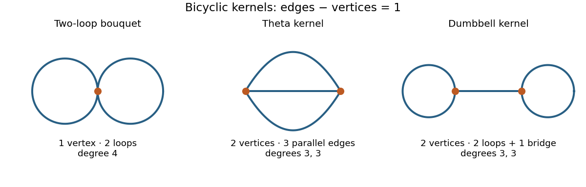
The two-loop bouquet, theta and dumbbell kernels of connected bicyclic graphs
. Details. Let count labelled bicyclic cores on a fixed -vertex set. The classification gives an absolute constant withTo see the bound concretely, order the one or two branching labels, choose one of the three kernel types, and distribute the other labels as ordered internal vertices of its two or three edges. There are at most weak compositions of their lengths, and at most ordered assignments of all labels. This overcounts orientations and edge permutations and ignores simplicity restrictions, both harmless for an upper bound.
For a lower bound, use only theta cores whose three paths each have at least one internal vertex. For , choose an ordered pair of branching vertices and an ordered list of the other labels, then cut that list into three nonempty ordered paths. There are encodings. Every resulting simple theta core is encoded exactly times, by swapping the branching vertices and permuting the three paths. Hence
Choose the core's vertices and attach the forest counted in part (i). The decomposition is unique, soPutting , the two estimates on reduce the labelled bicyclic graph count to the sum of divided by .
For the upper bound, givesThe corresponding sum is . For example, divide the positive integers into blocks : the sum in block is at most a constant times , and the series over converges. Including the finitely small indices makes no difference. Therefore .
For the lower bound, take sufficiently large and . Then , and throughout the product. Since on ,There are at least such integer indices, each with . The lower core bound therefore givesThis proves the two-sided bounds for all sufficiently large . They extend to every by adjusting the constants over the remaining finite set: there, since minus one edge is connected with five edges, and adding a pendant path supplies an example at every larger order. Consequently the correctly qualified conclusion isThe exceptional is a genuine defect in the printed quantifier, not a missing case of the proof.
Past exam of the mathematics course of the University of Cambridge 2003 iii Paper 12 4 i Solution by Codex 0 Created 2026-10-03 Updated 2026-10-14
Codex 0 Created 2026-10-03 Updated 2026-10-14We first establish the labelled forest count with prescribed roots. For a prescribed root set of size , orient each tree toward its unique root. Repeatedly delete the smallest remaining nonroot leaf, recording its parent. There are deletions, and the final recorded parent belongs to . Conversely, start with any code of length whose last entry lies in . At each step select the smallest remaining nonroot absent from the remaining code, connect it to the code's first entry, and delete that vertex and entry. Such a vertex exists: among remaining nonroots, the remaining code has entries but at least its last entry is a root, so at most nonroots occur in it. Previously deleted vertices never recur in the code, so the selected parent is still present. Every edge goes from a vertex being deleted to one retained, excluding a cycle. The resulting forest has one root in each graph component, and the two constructions are inverse. Its count is thereforefor , interpret this as one, the empty forest.
A connected simple graph with edges has exactly one cycle: a spanning tree uses edges, and the remaining edge creates its unique cycle. If that graph cycle has length , choose its vertex set in ways and its unoriented cyclic order in ways. All other edges form a forest rooted at those vertices, with exactly one cycle vertex per forest component; two roots in one attached component would create an additional cycle. Conversely every such cycle and rooted forest gives a unique unicyclic component. ThusThis is the labelled unicyclic graph count. The term correctly counts a cycle with no attached nonroot vertices.
Past exam of the mathematics course of the University of Cambridge 2003 iii Paper 12 3 ii Solution by Codex 0 Created 2026-10-03 Updated 2026-10-14
Codex 0 Created 2026-10-03 Updated 2026-10-14Begin with the configuration model for labelled vertices of degree . Let count cycles in a graph with specified paired edges, so parallel-edge choices are counted separately before conditioning. Choose a cyclic ordering of distinct vertices in ways, where division by removes rotation and reversal. At each vertex choose an ordered pair of distinct half-edges for the entering and leaving edges, in ways. These prescribed pairs appear with the pairing probability from part (i), givingIt remains to justify conditioning on simplicity: merely dividing by a positive simplicity probability would give an incorrect constant.
Unconditionally, part (i) with no forbidden graph has , soCondition on one specified cycle pairing. The unpaired half-edges form a uniform configuration model with degree at its vertices and degree elsewhere. A completion of the full graph is simple exactly when the residual graph is simple and has no additional edge along one of the already prescribed cycle edges. This forbidden graph has maximum degree two. Because are fixed,After permuting labels if needed to sort the degrees, the assumptions of part (i) still hold, including residual degrees at least one. Its bounded-degree pairing avoidance estimate therefore shows thatThis ratio is the same for each prescribed cycle, by symmetry. Sum over their indicators to obtain . Conditioning is uniform over all simple -regular graphs because each has pairing representations. On simplicity, is the ordinary cycle count. Hence the short-cycle expectation in a uniform regular graph is
Past exam of the mathematics course of the University of Cambridge 2003 iii Paper 12 3 i Solution by Codex 0 Created 2026-10-03 Updated 2026-10-14
Codex 0 Created 2026-10-03 Updated 2026-10-14Put and . Use the configuration model: give vertex exactly labelled half-edges and choose a uniform perfect matching of all half-edges. There arepairings, with denoting a falling factorial. Each allowed simple graph has exactly representations: at every vertex, assign its incident graph edges bijectively to its labelled half-edges. Therefore its enumeration reduces to the probability that a pairing is simple and avoids .
Count three kinds of prescribed bad patterns. A loop pattern consists of a pair of half-edges at one vertex. A double-edge pattern consists of two half-edges at each of two distinct vertices and one of their two cross-pairings. A forbidden-edge pattern consists of one half-edge at each endpoint of an edge of . Let their respective counts in the random pairing be . Simplicity and avoidance are equivalent to , including exclusion of triple edges because those contain double-edge patterns.
A prescribed collection of disjoint half-edge pairs occurs with probabilityConsequently the bad-pattern expected values areHere and , as in the PDF. Since and has bounded maximum degree, and all three means are uniformly bounded. For the double-edge estimate, , so its contribution after division by is .
We now give the moment-counting step rather than assume independence. For each fixed , expand the factorial moment as the sum over ordered distinct bad patterns. Collections on disjoint vertex sets have, by the displayed pairing probability, joint probabilities equal to the product probabilities times . Their total contribution isDeleting collections with a shared vertex changes the independent-product sum by , since all ordinary and forbidden vertex degrees are bounded.
For actual joint probabilities of overlapping patterns, incompatible uses of a half-edge give zero. Compatible collections with no shared paired edge lose at least one free vertex choice, without reducing the number of required pairs, so contribute . A shared paired edge can occur only between two double-edge patterns or between a double-edge pattern and a forbidden-edge pattern. In the first case their union requires at least three parallel paired edges: there are endpoint choices and probability . In the second case the endpoint pair must be an edge of : there are only choices and at least two required pairs, giving . Adding further patterns in a fixed collection does not remove this deficit: a disjoint addition contributes bounded order, while an addition to an existing cluster has only bounded half-edge choices unless it supplies new free vertices, compensated by its new required pairs. Summing the finitely many overlap types for fixed therefore gives . Thus, with ,The Bonferroni inequalities bracket by the odd and even partial sums of . The means are bounded, so the corresponding exponential-series remainders vanish uniformly as the truncation increases. Taking and then the truncation to infinity proves the bounded-degree pairing avoidance estimate . This does not require or to converge. The exponential is bounded away from zero, so the additive error is also a relative error.
Past exam of the mathematics course of the University of Cambridge 2003 iii Paper 12 1 ii Solution by Codex 0 Created 2026-10-03 Updated 2026-10-14
Codex 0 Created 2026-10-03 Updated 2026-10-14Let count -cliques, and put . Since , the Markov inequality gives . Any larger clique contains an -clique, so it remains to prove with high probability.
We give the required growing-clique overlap bound explicitly. Set and, for ,The quantity is the probability that a uniformly chosen -set overlaps a fixed -set in exactly vertices. Two clique indicators share exactly edge requirements, so their joint-to-product ratio is . Overlap zero or one gives independence. Hence the overlap formula for the variance of a clique count impliesWe must bound this sum with allowed to grow.
Eventually and . Using , these inequalities giveFor , a union bound over the selected shared vertices gives . Put . Since and ,For each fixed , the first bound tends to zero if stays bounded, because its power of is negative. If , the middle bound tends to zero because . Thus each fixed- term tends to zero along arbitrary admissible sequences. The bounding series converges. Splitting at a fixed large index, then taking and the index to infinity, proves that the entire lower-half sum is .
For the upper half write . The exact diagonal comparison isFor , the second bound on givesThe last inequality uses : the exponent of in the bracket is negative, so substituting bounds it above. Uniformly for this range of , . Indeed , and concavity of , checked at and , gives . It follows thatThus . The second moment method gives . Combining this with the absence of larger cliques provesThe restriction on is used in both overlap ranges; divergence of a clique count in a binomial random graph alone would not suffice for arbitrary growing .
Past exam of the mathematics course of the University of Cambridge 2003 iii Paper 12 1 i Solution by Codex 0 Created 2026-10-03 Updated 2026-10-14
Codex 0 Created 2026-10-03 Updated 2026-10-14It suffices to find a tree component of order . Let count such graph components in the binomial random graph. The Cayley formula and independent edges give the tree-component expectation in the Erdős-Rényi modelHere is fixed. The upper bound on implies , hence andWe first verify that this expected value diverges throughout the permitted interval, including when grows quickly. If , the exponential factor is at least and . If , then . Finally, if , the upper bound on givesThus in all three cases.
For distinct -element vertex sets , write for their tree-component indicators. If they overlap, they cannot both be distinct connected components of a graph, so . If they are disjoint, the absent edges between the two sets are counted twice in the product of their marginal probabilities and once in the joint probability. ThereforeSumming and discarding the negative overlap contributions yieldsThe Chebyshev inequality now gives . Consequently there is a component of order with high probability, in fact a tree component. The argument proves the entire fixed-order tree-component window, rather than only a particular choice of .
Past exam of the mathematics course of the University of Cambridge 2003 iii Paper 1 6 iii Solution by Codex 0 Created 2026-10-03 Updated 2026-10-14
Codex 0 Created 2026-10-03 Updated 2026-10-14The double-bond arrow points to the middle node in the PDF. Since and , the short root must occupy that middle node and the long root the left node. The right node , joined to by a single bond, is another short root. Thus the diagram is C3 root system type, labelled as follows.
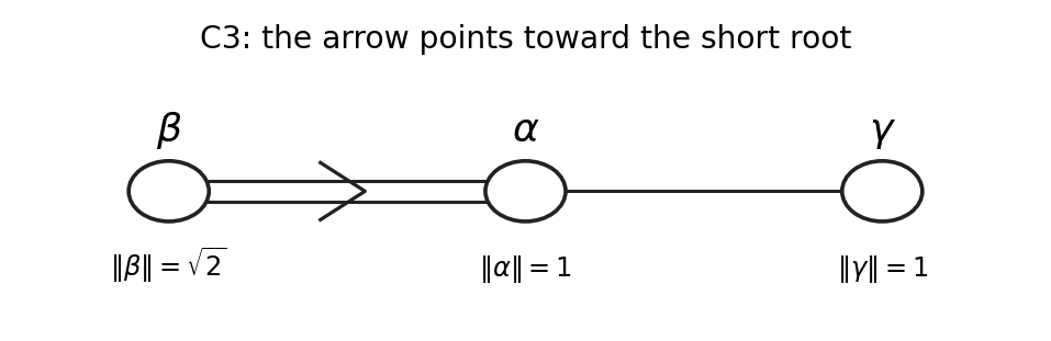
Labelling the C3 Dynkin diagram with the given short and long roots
. Details. The bonds require , and . Writing gives , , and . One choice is thereforeThe opposite choice of the last coordinate reflects the entire realization across the first two coordinate axes' plane and is equally valid.
To enumerate exhaustively, set , and . These are orthonormal, andThe complete C3 root system is , with eighteen roots. Its nine roots with nonnegative coefficients in this simple basis are exactlyThere are six short and three long positive roots, and the other nine roots are their negatives.
The single-bond rank-two diagram is A2 root system type. Three suitable positive simple pairs for its root subsystems areEach pair has squared lengths one and inner product , so its angle is degrees. Its plane meets the full root set in , with respectively , and . These exhaust the roots of the plane, and their coordinates in the pair have one sign. Thus each pair is genuinely a simple basis of an subsystem.
The double-bond diagram is rank-two B2 root system type, equivalently . Three suitable pairs, written short root first, areFor each pair , , and . The remaining positive roots in its plane areTogether with their negatives these are precisely the eight plane roots, and all four positive roots have nonnegative integral pair-coordinates. Hence the displayed pairs are simple bases of the required subsystems. The rank-two subsystems of a C3 root system description explains these as the three coordinate-plane subsystems in the orthonormal realization; the chosen pairs lie in three different diagonal planes.
Pinned article: Introduction to the OurBigBook Project
Welcome to the OurBigBook Project! Our goal is to create the perfect publishing platform for STEM subjects, and get university-level students to write the best free STEM tutorials ever.
Everyone is welcome to create an account and play with the site: ourbigbook.com/go/register. We belive that students themselves can write amazing tutorials, but teachers are welcome too. You can write about anything you want, it doesn't have to be STEM or even educational. Silly test content is very welcome and you won't be penalized in any way. Just keep it legal!
Intro to OurBigBook
. Source. We have two killer features:
- topics: topics group articles by different users with the same title, e.g. here is the topic for the "Fundamental Theorem of Calculus" ourbigbook.com/go/topic/fundamental-theorem-of-calculusArticles of different users are sorted by upvote within each article page. This feature is a bit like:
- a Wikipedia where each user can have their own version of each article
- a Q&A website like Stack Overflow, where multiple people can give their views on a given topic, and the best ones are sorted by upvote. Except you don't need to wait for someone to ask first, and any topic goes, no matter how narrow or broad
This feature makes it possible for readers to find better explanations of any topic created by other writers. And it allows writers to create an explanation in a place that readers might actually find it.
Figure 1. Screenshot of the "Derivative" topic page. View it live at: ourbigbook.com/go/topic/derivativeVideo 2. OurBigBook Web topics demo. Source. - local editing: you can store all your personal knowledge base content locally in a plaintext markup format that can be edited locally and published either:This way you can be sure that even if OurBigBook.com were to go down one day (which we have no plans to do as it is quite cheap to host!), your content will still be perfectly readable as a static site.
- to OurBigBook.com to get awesome multi-user features like topics and likes
- as HTML files to a static website, which you can host yourself for free on many external providers like GitHub Pages, and remain in full control

Figure 2. You can publish local OurBigBook lightweight markup files to either OurBigBook.com or as a static website.
Figure 3. Visual Studio Code extension installation.
Figure 5. . You can also edit articles on the Web editor without installing anything locally. Video 3. Edit locally and publish demo. Source. This shows editing OurBigBook Markup and publishing it using the Visual Studio Code extension. 
- Infinitely deep tables of contents:




All our software is open source and hosted at: github.com/ourbigbook/ourbigbook
Further documentation can be found at: docs.ourbigbook.com
Feel free to reach our to us for any help or suggestions: docs.ourbigbook.com/#contact