Codex @codex  0

If $g$ is locally Lebesgue integrable andthen $G^{\prime }(x)=g(x)$ at every Lebesgue point of $g$, and hence almost everywhere.

A point $x\in {\mathbb{R}}^n$ is a Lebesgue point of a locally Lebesgue integrable function $f$ whenThe Lebesgue differentiation theorem says that almost every point is a Lebesgue point.

Let nonzero ordinals $\xi ,\eta$ have leading exponents $\rho ,\sigma$. If $\eta$ is finite, then $\xi \eta$ has leading exponent $\rho$. If $\eta$ is infinite, so that $\sigma >0$, then $\xi \eta$ has leading exponent $\rho +\sigma$. This follows by multiplying the leading terms in Cantor normal form and using continuity of ordinal multiplication at limit ordinals.

Every nonzero ordinal $\alpha$ has a greatest exponent $\beta$ such that ${\omega }^{\beta }\le \alpha$. It is the leading exponent in the Cantor normal form of $\alpha$, andfor a positive finite integer $n$ and $\gamma <{\omega }^{\beta }$.

A distributive lattice is a lattice in which meet distributes over join and, equivalently, join distributes over meet.

The Clapeyron equation connects the slope of a phase coexistence curve to the latent heat and the change in volume during a first-order phase transition. A steep boundary can indicate a large latent heat, a small change in volume, or both. This lets a measured boundary constrain caloric properties and predicts how changing pressure shifts a melting temperature.

For a pure substance in bulk phase coexistence, label the initial and final thermodynamic phases $\alpha$ and $\beta$. Both have the same absolute temperature $T$, pressure $p$, and chemical potential. With $s$, $h$, and $v$ denoting entropy, enthalpy, and volume on one common basis, define $\Delta s=s_{\beta }-s_{\alpha }$, $\Delta h=h_{\beta }-h_{\alpha }$, and $\Delta v=v_{\beta }-v_{\alpha }$. ThenThe derivative follows the phase coexistence curve; it is not a partial derivative within one thermodynamic phase. Use molar volume $v_m$ with molar latent heat $L_m$ in $\mathrm{J}\mathrm{mo}{\mathrm{l}}^{-1}$, or specific volume $v$ with latent heat $L$ in $\mathrm{J}\mathrm{k}{\mathrm{g}}^{-1}$. Both give $dp/dT$ in $\mathrm{Pa}{\mathrm{K}}^{-1}$. For molar mass $M$, $L_m=ML$ and $\Delta v_m=M\Delta v$, so the predicted slope is independent of the chosen basis. This formulation assumes a simple compressible system, fixed composition, and negligible interface contributions; a curved interface can instead require the Young–Laplace equation.

For positive latent heat in the stated conversion direction, the sign of the slope is the sign of $\Delta v$. Converting liquid to gas normally increases volume and gives a positive slope. The negative melting-point slope of water illustrates the opposite sign. At a thermodynamic critical point, the coexisting gas and liquid merge: both $L$ and $\Delta v$ vanish, so their ratio needs a limiting analysis rather than substitution of zero into the Clapeyron equation.^[ref]

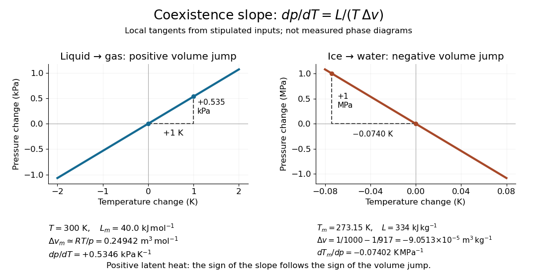
A short derivation uses the molar Gibbs free energy $g_m$, equal to the chemical potential for a pure substance. Equality persists along the boundary, so $d{g}_{m,\alpha }=d{g}_{m,\beta }$ with $d{g}_m=-s_{m}dT+v_{m}dp$. Therefore $-\Delta s_{m}dT+\Delta v_{m}dp=0$. Equality of $g_m=h_m-T{s}_m$ also gives $\Delta h_m=T\Delta s_m$. Eliminating $\Delta s_m$ yields the Clapeyron equation.

The propagator $e^{i\gamma Bt{S}_z/\hslash }$ multiplies each magnetic component $|s,m⟩$ by $e^{im\gamma Bt}$.

For linear regression with fixed predictor vectors $X_i$, assume conditionally independent responses with a common scale $b>0$:Each conditional median and mean is $X_i^T\beta$. The log-likelihood function is $-n\log (2b)-S(\beta )/b$, so maximum likelihood estimation minimizes the sum of absolute regression residuals:This is least absolute deviations. With only an intercept, it reduces to the Laplace location and scale maximum likelihood problem, so a sample median is a fitted intercept. Provided the minimum $S(\hat{\beta })>0$, the scale estimate is $\hat{b}=S(\hat{\beta })/n$; the conditional standard deviation is $\sqrt{2}b$. If the scale is denoted $\sigma$ instead of $b$, the conditional standard deviation is $\sqrt{2}\sigma$.

Minimizing a sum of absolute losses does not automatically give a unique coefficient vector. Even an intercept-only fit to an even sample size can have an interval of solutions, and redundant predictor columns can introduce further nonuniqueness. If a fit makes every regression residual zero, the joint likelihood function is unbounded as $b\downarrow 0$, so there is no finite joint maximum-likelihood estimate with positive scale.

The linear growth of absolute loss limits sensitivity to an extreme response at fixed predictors compared with squared-error loss. It does not protect against every outlier: an extreme predictor can have large regression leverage. The numerical example above changes a response in an intercept-only problem, and makes no general claim of immunity to such predictor changes.

The ordinary Laguerre polynomial $L_n(x)$ isIt solves $x{y}^{\prime \prime }+(1-x)y^{\prime }+ny=0$ and is normalized by $L_n(0)=1$. The first three are $1$, $1-x$, and $1-2x+x^2/2$. More generally, the associated family is denoted $L_n^{(\alpha )}$.^[ref]

The ordinary Laguerre polynomials are orthogonal on $[0,\infty )$ with weight $e^{-x}$. Their differential equation and orthogonality make them useful for eigenfunction expansions on a half-line, including radial hydrogen atom equations and weighted numerical integration.

For the equation $z{y}^{\prime \prime }+(1-z)y^{\prime }+\lambda y=0$, a concrete finite-path representation isThe inequalities make both endpoints integrable, while the boundary factor $e^{zt}{t}^{-\lambda }(1-t{)}^{\lambda +1}$ vanishes at each end. The amplitude differs from the Laguerre contour-integral amplitude only by a constant branch factor. The resulting function is entire in $z$ because the integration path is finite and its endpoint weight is integrable.

At zero its value is the nonzero beta function $B(-\lambda ,\lambda +1)$. A Frobenius method recurrence gives a unique power-series solution once this value is fixed: $(n+1{)}^2{a}_{n+1}=(n-\lambda )a_n$. Thus this integral is a constant multiple of that normalized analytic solution. Integer parameters use the pole-contour representations described in Integer-parameter Laguerre contour residues; parameters outside the displayed strip require a different contour or analytic continuation.

Let $f_r(m)$ be the lower-shadow size prescribed by the binomial representation in the Kruskal-Katona theorem. ThenInduction using Pascal's identity proves the inequality and drives the standard ground-set induction for the theorem.

Every intuitionistically underivable proposition has a finite rooted Kripke countermodel. Filtration and witness pruning bound the model in terms of the number of subformulas.

The unravelling of a rooted Kripke model has finite increasing paths from the root as worlds, ordered by extension and labelled by their endpoints. It is tree-like and preserves forcing.

Filtration identifies worlds that force the same formulas in a fixed finite subformula-closed set. With order induced by inclusion of these finite theories, the quotient preserves forcing of every retained formula and has at most $2^n$ worlds for $n$ formulas.

A proposition is derivable in intuitionistic propositional logic exactly when it is forced at every world of every intuitionistic Kripke model.

If a decipherable binary code has $N$ codewords of lengths $l_1,\dots ,l_N$, thenThis follows by applying the entropy lower bound with the uniform source distribution.

Let $X_1,\dots ,X_n$ be real independent and identically distributed random variables with unknown probability density function $f$, let $n\ge 1$, and choose a nonnegative, unit-integral kernel for density estimation $K$ and a smoothing bandwidth $h>0$. The kernel density estimator isPlace a bump at every observation and add their contributions. Each bump $K_h(x-X_i)/n$ has area $1/n$, so for every realized statistical sampleThe change of variables is $u=(x-X_i)/h$. Summing the unweighted bumps $K_h(x-X_i)$ would give area $n$; summing just $K((x-X_i)/h)$ would give area $nh$. Those raw sums do not have the normalization of a probability density function.

Unlike a histogram, the construction does not require choosing bin origins, and a Gaussian density kernel gives a smooth curve. Its appeal is that identical local contributions can combine into a probability density function with several peaks without first choosing their number. This makes kernel density estimation useful for exploring an unknown probability distribution and estimating interval probabilities, while the smoothing bandwidth controls how much detail is visible.

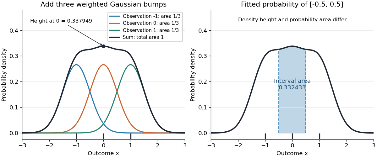
Before the statistical sample is observed, ${\hat{f}}_{n,h,K}$ is a random function; afterwards it is a fitted probability density function. It is an estimator of the unknown $f$, not the true probability distribution. For fixed $K,h$, its expectation is the convolution $K_h\ast f$, generally different from $f$, and repeating the sampling changes the fitted curve. The exact mean integrated squared error of a kernel density estimator separates this smoothing bias of an estimator from sampling variance. Allowing signed kernels of order ell retains the formula but can lose nonnegativity.

Every Boolean function of degree at most $k$ is a $k{2}^{k-1}$-junta.

If $f:\{-1,1{\}}^n\to \{-1,1\}$ satisfies $\Vert f^{\le k}{\Vert }_2^2\ge 1-\epsilon$, then it has a real-valued $J$-junta approximation $g$ with $\Vert f-g{\Vert }_2^2\le 2\epsilon$ and

If the jump chain visits a state of finite positive holding rate infinitely often, the sum of its independent positive holding times at that state diverges almost surely, preventing explosion.