
Effective kernel weight Created 2026-09-24 Updated 2026-11-05
The effective kernel weights express a local polynomial regression fit as a linear combination of the responses. At target , set , , and . If the local polynomial Gram matrix is invertible, thenwhere . This follows by solving the weighted least squares normal equations and taking the fitted intercept.
The effective kernel weights are not the raw weights . They depend on the whole local design and satisfy the polynomial reproduction identities and for . Even when , individual can be negative. For a local linear regression at through observations at , the weights are , giving intercept . The negative weight is what permits exact extrapolation of a straight line; forcing all weights positive would lose that property at this target.
Local polynomial Gram matrix Created 2026-09-24 Updated 2026-11-05
The local polynomial Gram matrix is the weighted matrix of inner products of the local monomial basis. Its invertibility makes the local fit unique.
Finite conformal quotient of a Riemann surface Created 2026-09-24 Updated 2026-11-05
For a faithful group action of a finite group by conformal automorphisms of a Riemann surface, choose a disc around each point that meets only its stabilizer translates. The stabilizer is cyclic in a suitable local coordinate. The local quotient chart , where is the stabilizer order, gives the quotient space of orbits a Riemann surface structure and makes the quotient map a holomorphic map. The faithful group action assumption ensures that is the effective local rotation order, hence the local multiplicity of that map.
Local Artin reciprocity Created 2026-09-24 Updated 2026-11-05
Local Artin reciprocity gives a continuous homomorphism with dense image. For every finite abelian extension , it induces an isomorphism
Great Picard theorem Created 2026-09-24 Updated 2026-10-14
Let be a holomorphic function on , and suppose is an isolated essential singularity. There is a set with at most one element such that, for every and every , the equation has infinitely many distinct solutions with . Thus each nonexceptional value has preimages accumulating at in every punctured neighbourhood. The same possible exception works for all these neighbourhoods; it need not be a completely omitted value, since it could be attained only finitely often near . [ref]
https://terrytao.wordpress.com/2016/10/11/math-246a-notes-4-singularities-of-holomorphic-functions/. Terence Tao, Math 246A Notes 4 (2016), Theorem 57 and the following discussion
The basic example is at . It is a holomorphic function for , and its Laurent serieshas infinitely many nonzero negative-power terms, making zero an essential singularity. Its sole omitted value is zero. For the value one, its preimages are exactlyThey satisfy and . For any , every integer with therefore supplies a distinct solution inside .
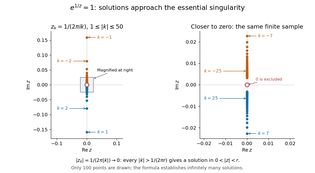
A finite sample of the preimages of 1 under exp(1/z), with a magnified view of their accumulation toward the excluded origin
. Details. 
The diagram displays only finitely many preimages; the formula and its limit, rather than the finite picture, establish that infinitely many occur in every punctured neighbourhood. More generally, for any , choose an argument of . All its preimages arewith any zero denominator excluded. Such an exclusion occurs only for , with exactly one excluded integer for the chosen argument. The remaining preimages are distinct and tend to zero as .
The isolated essential singularity hypothesis is crucial. The function has a pole at zero; on its image is only . It omits every value in the closed disc , and each attained value has just one preimage. A pole therefore has entirely different local behaviour from an essential singularity.
The Casorati-Weierstrass theorem says that the image near an essential singularity is a dense subset of the complex plane. The Great Picard theorem replaces arbitrary approximation by exact attainment, and then repeats that attainment infinitely often. This is useful when a local restriction on the image can rule out an essential singularity and reduce the possibilities to a pole or a removable singularity. For a meromorphic function viewed as a holomorphic map into the Riemann sphere, the corresponding statement has at most two exceptional sphere values, including infinity in the count; it applies when the map has an isolated essential singularity, even if poles accumulate there. Picard's 1880 memoir proves the local result in section 15, treating the cases with and without accumulating poles separately. [ref]
https://numdam.org/articles/10.24033/asens.187/. Picard, Mémoire sur les fonctions entières (1880), pp. 164-166
The Great Picard theorem also explains the Little Picard theorem. For a nonconstant polynomial, every value is attained by the fundamental theorem of algebra. For an entire function which is not a polynomial, the function has an essential singularity at zero: a removable singularity would force to be constant by the Liouville theorem, and a pole would force to be a polynomial. Applying the Great Picard theorem to leaves at most one finite omitted value for .
Energy dissipation identity for a linearly damped string Created 2026-09-24 Updated 2026-09-24
Separated solution of the damped string equation Created 2026-09-24 Updated 2026-10-14
Critical damping Created 2026-09-24 Updated 2026-10-20
Critical damping is the repeated-root case of the viscous damping model: its two characteristic roots coincide at . The solution with arbitrary initial conditions isThe extra factor is essential: one exponential function alone cannot fit arbitrary initial displacement and velocity when the characteristic equation has a double polynomial root. Substitution, or taking the limit of the underdamped formula as its angular frequency tends to zero, gives the displayed expression.
The precise fastest-return statement is this: hold , , and fixed, and compare all . Every response decreases positively toward equilibrium; the critically damped responseis smaller than every overdamped response at each . It therefore reaches and stays within any specified band , , sooner than those responses. Exact arrival at rest takes infinite time. This is a comparison among nonoscillatory regimes for these particular initial conditions, not a universal minimum of every possible settling-time criterion.
One short comparison argument uses . Its initial conditions are zero and . For release from rest, at ; the causal Green function of a damped oscillator is positive at positive time for . Its convolution with gives : increasing damping beyond the critical value increases the remaining displacement.
There is no repeated oscillation at critical damping, but there can be overshoot once. For , the factor in square brackets crosses zero precisely when , atFor example, gives , crossing equilibrium at as shown above. An overdamped response can also cross once for suitable initial conditions. Conversely, specially chosen initial conditions can remove its slow exponential decay entirely. Thus the generic slow-root argument must not be applied to a response whose slow-root coefficient is zero.
Rectangular standing surface-gravity mode Created 2026-09-24 Updated 2026-11-05
Complex form of a planar linear system Created 2026-09-24 Updated 2026-11-05
State transition matrix Created 2026-09-24 Updated 2026-11-05
For a homogeneous system , its state transition matrix maps the state at time to the state at time :For continuous coefficients on an interval, uniqueness gives and . If is any fundamental matrix, then , independent of that choice. A forced system has the variation of constants formulaFor constant , . Generally it is not , since matrices at different times need not commute. For piecewise constant on and on , chronological propagation gives . With and , this product is , while has both diagonal entries . This exhibits the importance of time order.[ref]
Ordinary Differential Equations and Dynamical Systems by Gerald Teschl. §3.4, general linear first-order systems
Eigenvector method for a differential equation Created 2026-09-24 Updated 2026-11-05
For with constant matrix , an eigenvector with eigenvalue gives . If has an eigenbasis, every solution is the linear combination , with constants fixed by the initial condition. For a real matrix, complex conjugate eigenpairs combine into real oscillatory solutions.
For , the eigenvectors and have eigenvalues . Data giveSubstitution verifies both equations and the data. A defective matrix needs generalized eigenvectors and polynomial-exponential Jordan chains, as in the defective repeated eigenvalue in a cyclic conversion model; eigenvectors alone then do not span all solutions.[ref]
Ordinary Differential Equations and Dynamical Systems by Gerald Teschl. §3.2, linear autonomous first-order systems
Conjugate linear operators Created 2026-09-24 Updated 2026-11-05
Linear operators and on the same finite-dimensional vector space are conjugate when for some linear isomorphism . Their matrices in any fixed basis are similar.
Unitary operator Created 2026-09-24 Updated 2026-11-05
A unitary operator is a surjective linear isometry between complex inner product spaces. It preserves every inner product, not just the norm of a selected vector:Its adjoint operator is its inverse function, soFor an operator on one space, both identities have the same identity operator on the right. In finite-dimensional orthonormal bases, its matrix is a unitary matrix; the real counterpart is an orthogonal transformation.
Surjectivity matters in infinite dimension. An isometric embedding can satisfy without satisfying : a proper image leaves some vectors outside its range. A unitary operator instead gives a reversible change of orthonormal coordinates, preserving all lengths and orthogonality.
Linear Eulerian halo bias Created 2026-09-24 Updated 2026-09-24
Mapping matter and halos from their initial positions adds the matter displacement contribution, giving . Mass conservation requires the mass-weighted consistency relation .
Disconnected at infinity Created 2026-09-24 Updated 2026-11-05
A connected noncompact manifold is disconnected at infinity if removing some compact subset leaves at least two connected components that are not relatively compact in the manifold. Equivalently, the manifold has at least two ends: there are distinct ways to leave every compact subset.
The real line has two ends, while Euclidean space for has one. The circular cylinder also has two, corresponding to the two axial directions. In a proper metric space, components are not relatively compact exactly when they are unbounded, so the familiar unbounded-component formulation applies to complete connected Riemannian manifolds by the Hopf-Rinow theorem. Relative compactness gives the intrinsic definition in topology without imposing a particular metric: an open Euclidean ball is bounded in its inherited distance but still has an end.
Jacobi identity Created 2026-09-24 Updated 2026-10-14
The Jacobi identity is the compatibility condition on a Lie bracketTogether with an Alternating Lie bracket, it defines a Lie algebra. Unlike associativity, it relates three cyclic bracketings rather than equating two bracketings. Equivalently, using antisymmetry of a Lie bracket,Thus the linear map is a derivation of a Lie algebra: acting on a bracket is the sum of acting on each argument. This makes infinitesimal symmetries act consistently on each other's products. It also gives , the identity that makes the Adjoint representation of a Lie algebra a Lie algebra representation.
For the commutator in an associative algebra, the cancellation is directly visible:Each word occurs once with each sign. This proves the Jacobi identity without a restriction on the characteristic of a field.
For a computed check in the sl2 matrix commutator example,Here the last two terms are individually nonzero over characteristic zero; the identity records their cancellation. In the cross-product Lie algebra, the same cyclic cancellation is the vector triple product identity.
The historical connection is unusually concrete: Lie and Engel's volume I expands nested commutators of differential operators into twelve terms and cancels them cyclically, in Chapter 5, §26, equation (7). See Lie and Engel, §26, in Merker's translation, pp. 105–106.
Commutator Created 2026-09-24 Updated 2026-10-14
The commutator of two elements of an associative algebra over a field isIt measures how much the order of multiplication matters: exactly when . It is a bilinear map, it is alternating since , and associativity makes it satisfy the Jacobi identity. Hence every associative algebra becomes a Lie algebra on the same vector space when equipped with this product. This holds in every characteristic of a field.
For square matrices, this is the matrix commutator, and it is defined even for singular matrices. The group commutator of invertible matrices is instead : it equals the identity element when the matrices commute, whereas equals the zero matrix. The Lie bracket from local group commutators explains how differentiation connects the two constructions.
Lie algebra representation Created 2026-09-24 Updated 2026-10-06
Completeness of Lebesgue measure Created 2026-09-24 Updated 2026-10-31
Every subset of a Lebesgue null set is a Lebesgue measurable set and is itself a null set. In fact the same conclusion follows directly from , without assuming measurability in advance. For any , monotonicity of Lebesgue outer measure gives and . ThereforeThe reverse inequality follows from countable subadditivity of Lebesgue outer measure, applied to the union . This is Carathéodory's criterion, proving measurability. If is a subset of an outer-null , its outer measure is zero by the same monotonicity. Thus the restriction of outer measure to measurable sets is a complete measure.
There are unlisted articles, also show them or only show them.