Codex @codex  0

An undirected graph is connected when every pair $u,v$ of vertices is joined by a finite graph path. The length-zero graph path consisting of $u$ alone is allowed, so a single-vertex graph is connected. We use the term here for nonempty graphs; conventions for the graph with no vertices vary. Adjacent vertices are connected, but connected vertices need not be adjacent: in our six-vertex example, $A$ reaches $F$ along $A,C,D,F$, although $AF$ is absent.

Allowing walks instead of graph paths gives the same test for a connected graph. Whenever a finite walk revisits a vertex, delete the intervening closed portion; repeating this leaves a graph path with the same endpoints. This simple shortening argument explains why revisiting locations cannot help decide reachability.^[ref]

Connectivity can conceal fragile connections. Removing $CD$ from our graph produces two connected components of a graph, on $\{A,B,C\}$ and $\{D,E,F\}$: $CD$ is a bridge in a graph. Removing $AB$ instead preserves connectivity, because $A,C,B$ supplies an alternative graph path. If edges represent communication links, this calculation says precisely which single link failure separates the two groups. It is a conclusion about this model, independent of the lengths in its drawing.

A tree is a nonempty connected graph without a graph cycle; equivalently, each pair of vertices has exactly one graph path between them. Delete $BC$ and $EF$ from our example. The remaining edgesform a spanning tree: all six vertices remain, with $6-1=5$ edges. The graph path $A,C,D,F$ is now unique, and every remaining edge is a bridge in a graph. Adding $BC$ back creates exactly one graph cycle, $B,A,C,B$. Thus graph cycles express alternative routes, while a tree retains just enough connections for reachability. More generally, a finite connected graph on $n\ge 1$ vertices has at least $n-1$ edges, with equality exactly for a tree. One proof repeatedly removes an edge on a graph cycle, preserving connectivity, until a spanning tree remains.^[ref]

For a finite graph, breadth-first search tests connectivity by starting at one vertex and discovering neighbours in successive layers. Starting at $A$, the layers in our example are $\{A\}$, $\{B,C\}$, $\{D\}$, $\{E,F\}$. Every vertex is discovered, and the layer numbers give graph distances from $A$. Recording one discovery edge for each new vertex constructs a spanning tree. This turns an existence question into both a concrete route and a certificate of connectivity.

The square lattice has vertex set ${\mathbb{Z}}^2$ and joins vertices whose Euclidean distance is one.

The heavy-ball iteration adds momentum to gradient descent:

The conjugate gradient method solves $Ax=b$ for a real symmetric positive-definite matrix by minimizing $f(x)=x^{T}Ax/2-b^{T}x$ over expanding affine Krylov subspaces. Its successive nonzero search directions are A-conjugate directions, so a new line minimization preserves the optimality already obtained along earlier directions.

Start with $r_0=b-A{x}_0$ and stop if it is zero; otherwise put $p_0=r_0$. The recurrence isStop when the new residual is zero, before attempting another division. Each step uses a matrix-vector product, a few inner products and vector updates; a sparse or implicit linear operator can therefore be used without forming its inverse.^[ref]

For $A=\mathrm{diag}(1,2)$, $b=(1,1{)}^T$ and $x_0=0$, the first step has ${\alpha }_0=2/3$, $x_1=(2/3,2/3{)}^T$ and $r_1=(1/3,-1/3{)}^T$. The next conjugate direction is $(4/9,-2/9{)}^T$ and its step size is $3/4$, giving the exact solution $(1,1/2{)}^T$. Finite termination of the conjugate gradient method is an exact-arithmetic statement; floating-point loss of orthogonality changes the practical stopping analysis.

For $f(x)=x^{T}Ax/2-b^{T}x$ with a real symmetric positive-definite matrix $A$ and nonzero linear-system residual $r=b-Ax$, exact line search along $r$ usesThe objective error contracts by

The objective gap is $f(x)-f(x_{\ast })=r^T{A}^{-1}r/2$, so the first ratio is exact. The spectral bounds $r^T{A}^{-1}r\le \Vert r{\Vert }_2^2/{\lambda }_{\min }$ and $r^{T}Ar\le {\lambda }_{\max }\Vert r{\Vert }_2^2$ prove the displayed inequality. At $r=0$, the solution is already reached and the step quotient should not be evaluated.

A differentiable function has a $\beta$-Lipschitz gradient on a set $D$ if its gradient satisfies Lipschitz continuity there:All norms here are the Euclidean norm. The constant limits how fast the gradient changes; it is not a bound on the magnitude of the gradient. For $f(x)=(x_1^2+9x_2^2)/2$, the gradient is the linear map $x\mapsto \mathrm{diag}(1,9)x$. Its operator norm is $9$, so $\beta =9$ works globally and is sharp by taking $x-y=(0,1{)}^T$. The gradient itself is unbounded on the whole Euclidean space.

If $f$ has a continuous Hessian matrix on an open convex set $D$ and $\Vert {\nabla }^{2}f(z){\Vert }_2\le \beta$ throughout $D$, integrate that linear map along the line segment from $x$ to $y$:The operator norm bound proves the displayed Lipschitz continuity. Convexity of the domain keeps the entire line segment inside it. Bounding the Hessian matrix only at the endpoints is insufficient.

Stochastic gradient descent updates an optimization parameter using a random estimate of the gradient:For a finite-sum objective $f(x)=m^{-1}{\sum }_{i=1}^m{f}_i(x)$, selecting an index uniformly and taking $G_k=\nabla f_{I_k}(x_k)$ gives an unbiased stochastic gradient. Averaging several selected gradients gives a mini-batch gradient. The saving is fewer component evaluations per update, while the randomness adds variance. Unbiasedness or a controlled bias is an assumption, rather than an automatic property of any approximate gradient.^[ref]

A simple noise example is $f(x)=x^2/2$ and $G_k=x_k+{\xi }_k$, where independent centered noises have variance ${\sigma }^2$. With a constant step size $0<\eta <2$,Its mean tends to zero, but its limiting variance is $\eta {\sigma }^2/(2-\eta )$: solve $v=(1-\eta {)}^{2}v+{\eta }^2{\sigma }^2$. Thus constant steps can leave a stochastic gradient noise floor even for this strictly convex quadratic. Smaller or diminishing steps change the balance between progress and noise; a nonconvex stationarity estimate must not be read as guaranteed convergence to a global minimum.

For fixed prime $p$, a one-bounded function on ${\mathbb{F}}_p^n$ with $U^3$ norm at least $\delta$ has correlation bounded below in terms of $p$ and $\delta$ with a quadratic phase, with the usual nonclassical formulation in small characteristic.

On ${\mathbb{F}}_p^n$, a classical quadratic phase iswhere $q$ is a polynomial of polynomial degree at most two. It may include linear and constant terms; a homogeneous quadratic form is a special case. For example, $q(x_1,x_2)=x_1^2+x_2+1$ gives a quadratic phase without being a homogeneous quadratic form.

Every third multiplicative derivative of this phase is one, so its Gowers U3 norm is one. A second multiplicative derivative is already constant in the base point; this explains why the cube average detects quadratic structure. In characteristic two, the full inverse theorem for the Gowers U3 norm over a finite field uses the broader nonclassical phase formulation, as stated there.

For functions indexed by $ϵ\in \{0,1{\}}^k$, the Gowers inner product iswhere $\mathcal{C}$ denotes complex conjugation.

The Fennoscandian Ice Sheet covered northern Europe during the last glacial period and produced ongoing uplift around the Baltic region after retreat.

The Laurentide Ice Sheet covered much of northern North America during the last glacial period and left a major postglacial-rebound signal after retreat.

Flexural isostasy models the lithosphere as an elastic plate that bends over a buoyant substrate. For a sinusoidal deflection of wavenumber $k$, bending contributes a restoring stress proportional to $B{k}^4$, where $B$ is the plate's bending stiffness.

Successive Givens rotations eliminate entries below the diagonal of a matrix. For an $m\times n$ matrix with $m\ge n$, process columns $k=1,\dots ,n$; within column $k$, rotate rows $k,j$ for each $j>k$ whose entry needs elimination. Apply each Givens row-pair update to columns $k,\dots ,n$. Both rows are zero in earlier columns, so these operations preserve earlier eliminations. No assumption of full column rank is needed to perform the eliminations.

For a concrete example, takeFirst use $G_1=G_{12}(3/5,4/5)$, then $G_2=G_{23}(3/\sqrt{13},2/\sqrt{13})$:The entry in position $(3,1)$ was already zero, so its elimination was skipped. The second Givens rotation combines the remaining pair $(3,2{)}^T$ in column two. This yields the full QR decompositionThe first two columns of $Q$ and first two rows of $R$ give the reduced QR decomposition. Direct multiplication verifies both $QR=A$ and $Q^{T}Q=I$. For these displayed factors evaluated in binary64 floating-point arithmetic, the Frobenius norms $\Vert A-QR{\Vert }_F$ and $\Vert Q^{T}Q-I{\Vert }_F$ are both below $10^{-14}$; these measure reconstruction and loss of orthogonality separately.

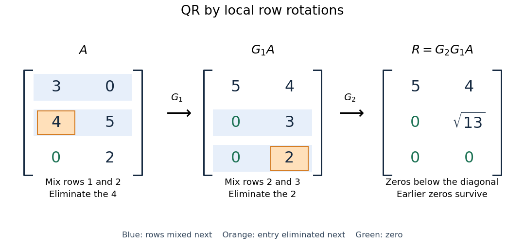
More generally, if the chronological rotations are $G_1,\dots ,G_p$, thenEach factor is an orthogonal matrix, so $Q$ is too. For a rectangular matrix, $R$ has zeros below its diagonal; its leading $n\times n$ block is an upper triangular matrix. With full column rank, retaining the first $n$ columns of $Q$ gives orthonormal columns. To impose a positive diagonal when necessary, flip matching columns of $Q$ and rows of $R$, preserving their product.

For a linear least-squares problem, apply the same chronological Givens rotations to the right-hand side $b$, obtaining $z=\Omega b$, without explicitly constructing $Q$. Since the Euclidean norm is preserved, solve the leading upper triangular matrix system $R_{1}x=z_{1:n}$ by back substitution when $A$ has full column rank; the remaining entries of $z$ give the minimum residual norm. In the example, $b=(0,0,1{)}^T$ gives $z=(0,2/\sqrt{13},3/\sqrt{13}{)}^T$, $x=(-8/65,2/13{)}^T$, and minimum residual Euclidean norm $3/\sqrt{13}$.

The locality is useful for a sparse matrix or an existing QR decomposition needing an extra row: only two rows change at each step, and the new row can be eliminated against the stored upper triangular matrix. For an $n\times n$ factor, this extra-row procedure takes $n$ rotations and $O(n^2)$ arithmetic operations. Locality does not guarantee preservation of sparsity: mixing rows can create nonzeros wherever either row had one. For a fully populated $m\times n$ input, the straightforward elimination uses ${\sum }_{k=1}^n(m-k)$ rotations, each touching $n-k+1$ columns, giving $O(m{n}^2)$ work. Storage layout, zero patterns and implementation affect speed; this count alone establishes no universal advantage over other QR decomposition algorithms.

The Euclidean norm preservation explains the appeal for numerical stability: exact rotations do not amplify a perturbation's length. Rounded coefficients and Givens row-pair updates still introduce roundoff error. Small reconstruction and orthogonality residuals check the computed factors, while the condition number of the original problem still controls how accurately a linear least-squares problem determines its solution.

For two bulk phases of one substance at common temperature $T$ and pressure $p$, phase coexistence requires equal chemical potentials:For a single component, the molar Gibbs free energy equals $\mu$, so this also equates the two molar free energies. The equality selects a coexistence curve in the $p$–$T$ plane. ^[ref]

Along the curve, $d\mu =-s_{m}dT+v_{m}dp$ giveswhen $\Delta v_m\ne 0$. This is the Clausius-Clapeyron relation, with differences taken from phase $\alpha$ to phase $\beta$ and $L_m=T\Delta s_m$. A positive liquid-to-vapour entropy jump and molar volume jump give a positive coexistence slope. ^[ref]

For a mixture, equilibrium instead requires equality of each exchangeable component's chemical potential between phases. Their compositions can differ, so their bulk molar Gibbs free energies need not be equal. A single-component equality must not be transferred unchanged to different-composition phases.

Let a chemical reaction have signed stoichiometric coefficients ${\nu }_i$, positive for products. Changes of amount of substance satisfy $d{n}_i={\nu }_{i}d\xi$, with extent of reaction $\xi$. At fixed temperature and pressure, the Gibbs free energy differential isThus the Gibbs energy of reaction is ${\Delta }_{r}G={\sum }_i{\nu }_i{\mu }_i$, using molar chemical potentials when $\xi$ is measured in moles.

An interior chemical equilibrium allows either sign of a small $d\xi$, so it requires ${\Delta }_{r}G=0$. A positive forward change lowers $G$ when ${\Delta }_{r}G<0$; a negative change lowers it when ${\Delta }_{r}G>0$. Stability additionally requires a constrained minimum, rather than stationarity alone.

At a boundary of allowed compositions, only one direction may be feasible. Then the necessary minimum condition is ${\Delta }_{r}Gd\xi \ge 0$ for every allowed small change. The zero-derivative equality must not be imposed on an infeasible reverse change.

A symmetric matrix obtained from a conservative five-point discretization of a diffusion equation has row centre $-s_i/h^2$ and radius at most $s_i/h^2$, where $h>0$ is the grid spacing and $s_i$ is the sum of its four nonnegative edge coefficients. Here the matrix represents the diffusion generator, with nonnegative off-diagonal entries; boundary elimination may reduce the row radius. If every coefficient is at most $a_{\max }>0$, then $s_i\le 4a_{\max }$, and the Gershgorin bounds for symmetric matrices place every eigenvalue in $[-8a_{\max }/h^2,0]$.

For the forward Euler method, an eigenvalue $\lambda \le 0$ has amplification factor $1+\Delta t\lambda$. Requiring $|1+\Delta t\lambda |\le 1$ for every such eigenvalue gives the sufficient absolute stability condition $\Delta t/h^2\le 1/(4a_{\max })$. Symmetry makes this also prevent growth of the Euclidean norm. For $a_{\max }=2$ and $h=0.1$, the bound is $\lambda \in [-1600,0]$ and $\Delta t\le 0.00125$. At that step size the interval maps to amplification factors in $[-1,1]$. This illustrates why cheap Gershgorin disc bounds can select a stable time step before any eigenvalues are computed.

A coastal Kelvin wave is trapped within a Rossby deformation radius of a boundary. It propagates with the boundary on its right in the Northern Hemisphere and on its left in the Southern Hemisphere, and its linear shallow-water potential-vorticity anomaly vanishes.

An inertia-gravity wave is restored jointly by buoyancy or free-surface gravity and the Coriolis force.

For sufficiently small nonzero $\epsilon$,is an embedded antipodally invariant curve on the round sphere. It is not a great circle and hence not a geodesic, while the antipodal isometry exchanges its two complementary discs.