
Charged particle in a uniform magnetic field Created 2026-09-24 Updated 2026-11-05
Relativistic Lorentz force Created 2026-09-24 Updated 2026-10-03
gives and .
Proca equation Created 2026-09-24 Updated 2026-11-05
With Minkowski metric signature and source coupling added to the Proca action, a massive vector field coupled to a conserved current obeysIn vacuum this gives after imposing the dynamically derived Lorenz constraint in Proca theory. The explicit mass term breaks the gauge invariance of the massless Maxwell theory.
Maxwell stress tensor Created 2026-09-24 Updated 2026-11-05
Magnetic spherical-shell matching Created 2026-09-24 Updated 2026-11-05
Across an interface with no free surface current, the normal component of and tangential component of are continuous. For an axisymmetric spherical shell, harmonic scalar potentials have dipole form in each radial region.
Bound charge and bound current Created 2026-09-24 Updated 2026-11-05
Polarization and magnetization produce the effective sourcesDefining and moves these sources into the macroscopic fields.
Inductance Created 2026-09-24 Updated 2026-10-13
Inductance relates electric currents to the magnetic flux linkage they produce. For a single linear coil with fixed geometry and magnetic response, its self-inductance is the constant inHere is magnetic flux linkage from the coil's own electric current . The SI unit of inductance is the henry. Knowing inductance lets us predict the induced electromotive force when electric current changes, and the magnetic energy stored by an inductor. [ref].
For example, a coil of self-inductance carrying electric current has magnetic flux linkage . If its turns link the same magnetic flux, each turn has magnetic flux . Keeping the geometry and magnetic response fixed while doubling electric current doubles magnetic flux linkage and quadruples the inductor's magnetic energy.
The comparison with capacitance is useful: a linear capacitor has and stores capacitor energy in its electric field, whereas a linear inductor has and stores magnetic energy in its magnetic field. The RLC circuit brings both forms of energy storage together.
Capacitance Created 2026-09-24 Updated 2026-10-18
The capacitance of a linear two-terminal capacitor is the constant relating its separated electric charge to its terminal electric potential difference:Here is the electric charge on one electrical conductor, the other carries , and is their electric potential difference with the same ordering. Reversing the terminal ordering reverses both and and leaves capacitance unchanged. An ideal passive capacitor has ; an ordinary pair of separated electrical conductors with positive permittivity has . At , use rather than the undefined ratio .
For example, electric charge magnitude at terminal electric potential difference gives capacitance . At , the same linear capacitor has and the same capacitance. The plots in capacitor energy show that capacitance is the slope of the electric charge versus terminal electric potential difference graph.
For fixed geometry and linear material response, capacitance depends on dimensions and permittivity, rather than the source's terminal electric potential difference. This is why capacitance is a useful property of a component: once it is known, predicts the separated electric charge for each operating terminal electric potential difference. The SI unit is the farad, . [ref].
For combinations of capacitors, the same terminal definition gives an equivalent capacitance. Two identical capacitors of capacitance connected in parallel share the same terminal electric potential difference, and their electric charges add, giving . Connected in series with an initially neutral isolated junction, they carry equal plate electric charge magnitudes and their terminal electric potential differences add, giving . [ref].
Magnetic field Created 2026-09-24 Updated 2026-10-13
A magnetic field is a vector field whose local value determines the magnetic part of the Lorentz force on a body with electric charge and velocity . In SI units,where is the speed, , and is the angle between the velocity and the magnetic field. The cross product makes a nonzero magnetic force perpendicular to both the velocity and the magnetic field. The right-hand rule gives its direction for positive electric charge; negative electric charge reverses it. [ref].
The SI unit of magnetic field is the tesla:For a stipulated example in SI units, take electric charge , velocity , and magnetic field . The cross product gives magnetic force . With the same speed directed along , the magnetic force is zero: motion parallel to a magnetic field produces no magnetic acceleration.
Magnetic field lines visualize the direction of a magnetic field by being tangent to it at each point. They are not generally the path of a body with electric charge: in a uniform magnetic field along , the magnetic field lines are straight while transverse velocity produces circular motion, and adding parallel velocity produces helical motion in a uniform magnetic field. The worked Lorentz force example below illustrates this distinction.
A magnetic field need not be static. Magnetostatics is the restricted case with no dependence on time; an electromagnetic wave has changing electric field and magnetic field even in vacuum. A changing magnetic field is coupled to the electric field through Faraday's law of induction. [ref]
https://www.feynmanlectures.caltech.edu/II_20.html. Feynman lectures, II.20: electromagnetic waves in free space
. The useful separation is between local bending, described by the Lorentz force, and the amount of magnetic field crossing a surface, described by magnetic flux. Electric field Created 2026-09-24 Updated 2026-11-05
The electric field gives the electric force per unit test electric charge: for a stationary test particle. Its direction is the force direction for a positive test charge, while a negative charge experiences the opposite force. The field is defined by the source configuration, not by the sign chosen for the probe.
A sufficiently small test charge samples the field without significantly disturbing the sources. In electrostatics, relates it to the electric potential; mapping equipotentials therefore determines field directions and magnitudes. A moving charge can also experience a magnetic force, so the complete Lorentz force cannot generally be represented by alone.
Electric charge Created 2026-09-24 Updated 2026-10-20
Electric charge is an additive, signed property of matter that determines its coupling to the electromagnetic field. Write a particle's electric charge as , or a collection's total electric charge as ; the SI unit is the coulomb, . A stationary test particle in an electric field experiences electric force , while motion adds the magnetic part of the Lorentz force. Electric charge both produces an electric field and determines the response to one. For two stationary point particles in vacuum, Coulomb's law makes like signs repel and opposite signs attract. The choice of which sign to call positive is a convention, used consistently: protons carry and electrons carry , where is the elementary charge. [ref]
https://www.feynmanlectures.caltech.edu/II_01.html. Feynman, Leighton and Sands, II.1: electrical forces, fields and the Lorentz force
.Additivity means adding signed electric charges, rather than their magnitudes:for ordinary matter containing protons, electrons, and electrically neutral neutrons. A toy collection with seven protons and ten electrons has , however much neutral material accompanies it. Charge neutrality means ; it does not mean an absence of charged constituents. Nor does it guarantee an absence of electric force: the spatial arrangement of positive and negative electric charges matters, as illustrated by an electric dipole. This makes a tiny imbalance in an otherwise nearly neutral object physically important. [ref]
https://www.feynmanlectures.caltech.edu/II_01.html#Ch1-S1. Feynman, Leighton and Sands, II.1.1: neutrality, imbalance and residual electrical forces
.Charge conservation states that a collection closed to transport of electric charge keeps its total signed . If electrons move from object A to object B without other exchange, then and ; the sum is unchanged. The amount of positive electric charge alone need not be conserved: creation of an electron and a Positron adds opposite electric charges with zero sum. These bookkeeping rules let us distinguish separation or transport of electric charge from creation of net electric charge. [ref]
https://www.feynmanlectures.caltech.edu/I_04.html#Ch4-S4. Feynman, Leighton and Sands, I.4.4: conservation of net charge
.A simple motivating experiment uses two charge-producing paddles, a conducting pail on an insulating support, a grounded outer shield and a high-input-impedance electrometer. Zero the pail, then isolate it. Rub the initially neutral paddles together, keeping their charged surfaces away from other objects. Lower each deeply into the pail without touching: the electrometer gives opposite signs. Inserting both together tests cancellation. For a separate contact test, insert one charged paddle without touching and withdraw it: the reading returns to zero. Repeat after zeroing, this time touching the inner wall before withdrawal: a residual reading shows transfer of electric charge. Zero the pail and reinsert the paddle to test how much electric charge remains on it. PASCO describes these procedures in Basic Electrostatics System manual, demonstrations 1A and 1B, printed pp. 13–16.
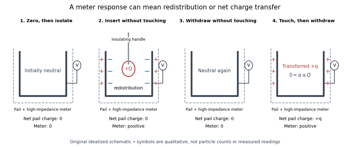
Electric charge redistribution versus transfer in a conducting pail
. Original qualitative schematic for a positively charged inserted object. Without contact, electrostatic induction separates negative inner-surface and positive outer-surface electric charges, while the pail's total remains zero. Contact can leave net positive electric charge after withdrawal. Symbols are not particle counts; no measured readings are plotted. Source. Details.
The crucial control is withdrawal without contact: a response during insertion can come from electrostatic induction, which redistributes the pail's existing electric charge. In the fixed-geometry approximation, the electrometer measures electric potential difference proportional to enclosed electric charge, with conversion set by effective capacitance; a voltage reading is not already a measurement in coulombs. Opposite readings and their cancellation test additivity and charge conservation within resolution. Leakage or accidental contact spoils that interpretation, and contact need not transfer all the paddle's electric charge. This macroscopic experiment cannot resolve elementary charge steps: that requires the much smaller particles of the oil drop experiment.
Right-hand rule Created 2026-09-24 Updated 2026-11-05
The right-hand rule fixes the orientation of a cross product and relates the circulation direction of an electric current to the direction of its magnetic field.
Effective potential stability criterion Created 2026-09-24 Updated 2026-09-29
After reducing conserved cyclic momenta, an equilibrium at a strict local minimum of the resulting effective potential is stable in the reduced one-degree-of-freedom dynamics.
Positively invariant set Created 2026-09-24 Updated 2026-10-13
Lyapunov function Created 2026-09-24 Updated 2026-11-05
A Lyapunov function near an equilibrium point is a continuously differentiable scalar with , for nearby , and nonpositive orbital derivativeIts sublevel sets act as nested barriers: a trajectory cannot cross from a lower value to a higher one. The First Lyapunov theorem uses these barriers to prove Lyapunov stability without an explicit solution.
For , choose ; then away from zero and trajectories converge to the equilibrium. For the planar rotation , , the choice instead has . It proves stability, but trajectories remain on circles and do not converge.
Thus a nonpositive derivative alone does not establish asymptotic stability. Strict negativity, or an argument such as LaSalle's invariance principle controlling the invariant part of the zero-derivative set, supplies the missing information. A Lyapunov functional applies the same idea to a whole function-valued state.
Basin of attraction Created 2026-09-24 Updated 2026-11-05
The basin of attraction of an attracting state or set consists of the initial states whose forward trajectories approach it. A basin is a subset of state space, so its boundary can separate physically different long-term outcomes even when the same equations and parameters apply everywhere.
For , positive initial values converge to and negative values converge to . The sign of points toward the corresponding outer equilibrium on either side, and uniqueness prevents crossing the invariant state . Thus the basins are and , with the unstable equilibrium as their boundary. Small fluctuations near a basin boundary can change the eventual outcome, while equal-size perturbations deep inside a basin may have little lasting effect. This is a geometric reason to distinguish local stability from global selection.
Equilibrium of an autonomous differential equation Created 2026-09-24 Updated 2026-10-03
An equilibrium is a state where the autonomous vector field vanishes.
Unstable equilibrium Created 2026-09-24 Updated 2026-09-24
An equilibrium is unstable when arbitrarily small perturbations can move trajectories away from it.
Resonance Created 2026-09-24 Updated 2026-11-05
Resonance is enhanced response when a periodic drive couples efficiently to a system's natural oscillatory motion. The drive must have a nonzero projection onto the relevant mode; matching a natural frequency alone is insufficient if the forcing pattern cannot excite that mode.
For with , the steady displacement amplitude isWeak damping gives a large response near , while damping limits the amplitude and permits a repeatable steady response after transients decay. A frequency sweep of the drive tests both response magnitude and phase lag. The exact peak depends on which observable is measured: displacement amplitude and absorbed power need not peak at precisely the same frequency. In the undamped resonant idealization with effective forcing, the amplitude grows instead of approaching a bounded steady oscillation.
Fixed point stability for an iteration Created 2026-09-24 Updated 2026-11-05
For a scalar iteration , a fixed point satisfies . A small deviation obeys , so gives local asymptotic stability and gives local instability when the map is differentiable nearby.
The multiplier's sign also describes the approach. A positive multiplier below one preserves the sign of sufficiently small deviations, while a negative multiplier of magnitude below one makes successive deviations alternate around the fixed point. For example, converges while changing sign at each step. At multiplier magnitude one, higher-order terms can decide the outcome, so the strict test is inconclusive. This differs from the sign-of-real-part condition for a continuous-time autonomous differential equation; an iteration advances by finite steps.
There are unlisted articles, also show them or only show them.