
Horizon problem Created 2026-09-24 Updated 2026-11-05
In a decelerating hot Big Bang model, widely separated regions of the observable universe have nearly equal conditions despite having no shared past light cone. Inflation supplies an earlier era with a shrinking comoving Hubble radius, allowing a formerly causal patch to grow beyond the later horizon.
Critical density Created 2026-09-24 Updated 2026-11-05
At a specified Hubble parameter , the critical energy density isThe Friedmann equation sets the spatial-curvature term to zero when the total energy density, including any cosmological constant contribution, equals this value. Dividing by gives the corresponding critical mass density . Confusing these two conventions loses a factor of .[ref]
The cosmological density parameter compares one component with this geometric normalization at the same epoch. Spatial flatness requires the sum of the component cosmological density parameters to be one, rather than each component separately. Since changes with , a constant energy density need not have a constant cosmological density parameter.
The criterion concerns spatial geometry in an FLRW metric. It does not alone determine the future lifetime of an expanding universe: pressure and dark energy affect its subsequent dynamics. It also differs from critical densities defined by phase transitions or plasma processes.
Cosmological perfect-fluid continuity equation Created 2026-09-24 Updated 2026-09-28
For a homogeneous fluid of energy density , pressure , and scale factor , adiabatic work in a comoving volume gives
Transfer function Created 2026-09-24 Updated 2026-10-13
A transfer function packages the response of a linear time-invariant system into a rule for turning a plant input into a plant output. Instead of solving a differential equation separately for every signal, take a Laplace transform, multiply by , then transform back. This also makes it possible to compare slow and fast oscillations through the continuous-time frequency response.
Here consider a continuous-time, causal, finite-dimensional linear time-invariant system with one plant input and one plant output . With every initial state set to zero, its transfer function is defined byThe ratio is used where in a common Laplace convergence region; describes the system, independently of that particular plant input. Zero initial state matters: stored motion or another nonzero initial condition can contribute to the plant output even when the plant input vanishes. [ref]
The first-order low-pass filter below shows the same transfer function predicting both a step and a sustained sinusoid. Its pole gives a decay rate, its value at zero gives the eventual gain, and its values along the imaginary axis give the continuous-time frequency response. These descriptions make a useful bridge between a physical relaxation model and control theory calculations.
Burgers vortex Created 2026-09-24 Updated 2026-11-05
A Burgers vortex is a steady rotating flow in which axial stretching intensifies vorticity while viscosity spreads it outward. Choose cylindrical coordinates with imposed axial strain rate :Here is kinematic viscosity and is the total circulation. The radial inflow and axial outflow preserve volume. Integrating the vorticity over a disk gives the swirl velocityThe centre is regular, while outside the core the swirl approaches that of a line vortex.[ref]
The core radius scales as : stronger imposed stretching narrows the core, while stronger viscosity broadens it. This exact idealization illustrates a competition important in turbulence, but does not imply that every turbulent vortex is steady or has a Gaussian profile. Its sustaining strain is externally imposed; the swirl is not an isolated flow evolving without that environment.
Acoustic energy flux Created 2026-09-24 Updated 2026-11-05
The acoustic energy flux is the rate at which a small-amplitude acoustic wave transports energy through oriented unit area. For pressure perturbation and particle velocity , its leading instantaneous value is . Averaging over a cycle gives sound intensity.
With physical fields represented by real parts of and , the cycle average isThe relative wave phase matters: large pressure alone does not imply large transported power. In a progressive plane acoustic wave, pressure and longitudinal velocity are in phase, and . In a perfect standing wave they are in phase quadrature locally, giving zero net cycle-averaged transport despite stored acoustic energy. Simultaneous measurements of pressure and particle velocity can distinguish the two situations.
Falkner-Skan equation Created 2026-09-24 Updated 2026-11-05
The Falkner-Skan equation is a similarity reduction of the steady two-dimensional boundary-layer equations when the imposed outer speed isChoose the streamfunction and similarity coordinatewith kinematic viscosity . Then and automatically satisfy incompressibility.
The streamwise equation reduces towhere primes differentiate with respect to . An impermeable stationary no-slip wall and matching to the outer flow giveThus is the streamwise speed divided by the local outer speed.
At , the outer speed is constant and the equation becomes the Blasius equation. Positive gives an accelerating outer flow and decreasing outer pressure, since ; negative gives an adverse pressure gradient. The equation and boundary conditions determine a Falkner-Skan boundary layer, rather than a generic profile independent of the imposed pressure field.
Boundary layer Created 2026-09-24 Updated 2026-10-14
A boundary layer is a thin region next to a surface in which viscosity remains significant even when inertia dominates the outer fluid flow. Its simplest example is laminar flow along a stationary flat plate: the no-slip boundary condition imposes zero velocity at the plate, while the outer velocity is . The resulting thin velocity profile contains a large normal velocity gradient, so small dynamic viscosity can still produce appreciable wall shear stress. The Blasius boundary layer makes this competition quantitative and explains how a plate aligned with the incoming fluid flow acquires drag.
The same balance appears in a singular perturbation of a differential equation: large derivatives in a thin region can keep a term with a small coefficient significant. For on with and , the inner variable resolves a left boundary layer of width .
Rayleigh-Taylor instability Created 2026-09-24 Updated 2026-11-05
Rayleigh-Taylor instability occurs when the effective acceleration places a denser fluid above a lighter one so that small interface disturbances can release gravitational potential energy. A downward bulge of dense fluid tends to sink while adjacent lighter fluid rises. The inertia of the moving fluids determines how rapidly the disturbance grows.
For two deep inviscid incompressible fluids at rest, with upper mass density and no surface tension, a sinusoidal disturbance of horizontal wavenumber has growth rateIncluding constant surface tension subtracts from the right-hand side, stabilizing sufficiently short wavelengths.[ref]
Fluid Mechanics by David Tong. Rayleigh-Taylor Instability, author-hosted fluids4.pdf, §5.1.4, printed pp. 190–191: stationary two-fluid dispersion relation and capillary cutoff
The assumptions exclude finite-depth boundaries, viscosity and diffuse interfaces. An idealized two-layer experiment records the interface height after a small imposed disturbance; its early exponential growth can test the linear prediction before the interface rolls into large plumes. Material derivative Created 2026-09-24 Updated 2026-11-05
The material derivative measures change seen by a moving material parcel rather than by an observer fixed in space. For a scalar field and a Lagrangian trajectory satisfying , the chain rule gives .
For steady in a one-dimensional flow with constant velocity , the fixed-position derivative vanishes but . The parcel experiences change because it crosses a spatial gradient. This advection term explains why a steady velocity field can still produce parcel acceleration. [ref]
Mass conservation Created 2026-09-24 Updated 2026-11-05
Mass conservation requires that a material region retain its mass when no mass-producing process is included. For mass density and velocity field , the local continuity equation isor equivalently . The second form says that a moving fluid element loses mass density as its volume expands, rather than losing mass.
A pipe narrowing in a steady flow gives a simple test: the mass flow through every cross-section is the same, so is constant for a uniform section profile. Constant mass density then makes constant. In Lagrangian coordinates, the equivalent relation is , where is the local volume ratio. A fixed observation region can gain mass through its boundary even though the material moving through it obeys mass conservation.
Continuity equation Created 2026-09-24 Updated 2026-11-05
A continuity equation expresses local conservation by balancing density changes against flux divergence. For mass density transported with fluid velocity and no mass sources, it is .
Expanding the divergence gives , where is the material derivative. A fluid parcel can change density when the surrounding flow compresses or expands it. For constant nonzero density, the equation reduces to the incompressibility condition .
In a steady one-dimensional pipe flow, integrating across a section gives constant mass flow rate , under the usual uniform-section approximation. Velocity need not remain constant when the density or channel area changes; the continuity equation constrains their product.
Energy flux Created 2026-09-24 Updated 2026-11-05
An energy flux describes transport of energy across a surface. A flux density has units of power per area; the total outward power through is , with outward unit normal . A local conservation law relates the divergence of to the time derivative of the energy density and any sources.
For a one-dimensional inviscid gas with velocity , pressure , mass density and internal energy density , the total mechanical-plus-internal energy flux isThe first two terms advect internal energy and kinetic energy. The term is pressure work: a moving section of area transmits force at velocity , giving power . This formula assumes negligible viscous stress and heat conduction; those processes contribute their own energy-transfer terms when retained.
Momentum flux Created 2026-09-24 Updated 2026-09-24
Mass flux Created 2026-09-24 Updated 2026-10-13
Compton scattering Created 2026-09-24 Updated 2026-10-20
Compton scattering redistributes photon energy and momentum in a collision with a charged subatomic particle, here an electron. For a free electron initially at rest in the chosen inertial frame, an incident photon of energy leaves with energy after deflection through . The angle is between the incident and outgoing photon directions; it is not the electron recoil angle. Four-momentum conservation giveswhere is the electron rest mass and its final kinetic energy. The photon energy loss pays for the electron recoil: neither energy nor momentum disappears.
For an original worked example, stipulate , the rounded electron rest energy , and the rounded Compton wavelength ; means electronvolts. Treat these rounded inputs as the example's constants. They give the following calculated values, with energies rounded to three decimal places:
| Photon deflection | Outgoing photon energy in | Electron kinetic energy in | Wavelength increase in |
|---|
Since , every outgoing photon has and . At zero deflection there is no recoil; backscattering transfers the most energy. At fixed , the absolute wavelength increase is independent of incident energy, while the fractional energy loss grows with . This makes Compton scattering useful for inferring energy transfers from directions in photon detectors.
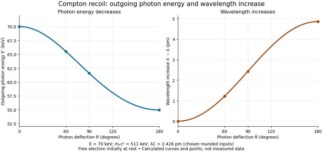

The free-electron-at-rest assumption matters. An electron in a bound state has binding energy and an initial momentum distribution. Neglecting these is useful when the transferred energy is large compared with the relevant binding energy and the initial momentum is small compared with the resolved momentum transfer. Otherwise the outgoing photon energies can broaden or depart from the stationary-target formula; an initially moving electron can even give energy to the photon.
A material may also scatter X-rays through a coherent elastic scattering channel with an effectively unshifted component. When an intact chemical atom of mass takes the recoil, the corresponding Compton wavelength is much smaller than the electron value. The single free-electron curve does not predict that component's weight. More generally, energy versus angle is a kinematic constraint; angular wave intensity requires a differential scattering cross-section, together with target and detector information.
Ramsey theory Created 2026-09-24 Updated 2026-10-13
Ramsey theory studies configurations that every finite coloring of a sufficiently large structure must contain. Its striking message is that some order is unavoidable even when no organized construction was used. A basic example is the Ramsey number for triangles: color every edge of a complete graph on six vertices red or blue, in any way, and some triangle in a graph has all three edges the same color. Five vertices do not suffice.
The objects receiving colors matter. In the Ramsey number for triangles, colors belong to edges, which represent all unordered pairs of distinct vertices; the vertices themselves have no colors. In the finite Ramsey theorem, colors can instead belong to all -element subsets of a finite set. A monochromatic set or homogeneous set for a colouring expresses agreement among the appropriate colored objects.
Why is this useful? Ramsey theory provides existence guarantees in combinatorics that survive every possible assignment of a fixed finite number of colors. The Ramsey theorem turns this into a structural dichotomy: every sufficiently large graph contains a large clique or a large independent set. In arithmetic, the Van der Waerden theorem guarantees monochromatic arithmetic progressions. The beauty is the universal quantifier: an adversary can choose every color and still cannot prevent the promised configuration.
These guarantees concern precisely specified configurations under stated hypotheses. They do not justify selecting arbitrary patterns in empirical data after seeing the data, or attributing statistical significance to a selected pattern. A mathematical guarantee of some monochromatic configuration alone says nothing about the empirical meaning of that configuration.
The subject's name comes from F. P. Ramsey's [ref]. The [ref]
https://www.cs.umd.edu/~gasarch/BLOGPAPERS/ramseyorig.pdf. original paper, pp. 264-268, Theorems A and B
records receipt on 28 November 1928 and presentation on 13 December 1928. Ramsey introduced the Ramsey theorem for r-sets and finite Ramsey theorem as tools for a problem in mathematical logic, while recognizing their independent interest in combinatorics. He also distinguished proving that a finite threshold exists from finding its smallest value, the quantitative question captured by a Ramsey number. Analysis of Boolean functions Created 2026-09-24 Updated 2026-09-24
Analysis of Boolean functions studies real-valued functions on a Boolean hypercube using Fourier analysis, probability theory, and combinatorics.
Permutation Created 2026-09-24 Updated 2026-10-13
A permutation of a set is a bijection : every element has exactly one image and every element appears exactly once as an image. For a finite set, a permutation can also be recorded as an ordering of all its elements, once a reference order has been chosen. For three distinct letters , the six orderings areThere are three choices for the first letter, two unused letters for the second, and one for the third. Every path in the tree gives one complete ordering, and every ordering has one such path, so the rule of product gives , a factorial.
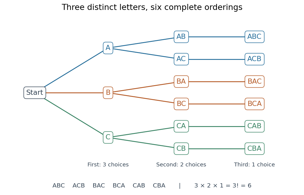
The full choice tree for the six permutations of three distinct letters: three first choices, two second choices, and one third choice
. Details. 
Ordering versus mapping. Label the reference positions . An ordering tuple of these labels describes the function ; conversely, reading the images recovers the ordering. For example,means , , , . Its ordered image list is , whereas its cycle decomposition of a permutation is : starting at , follow its successive images back to . Parentheses in the latter expression encode arrows around a permutation cycle, rather than an image list in reference order. [ref]
https://math.mit.edu/~fgotti/docs/Courses/C.%20Combinatorial%20Analysis/11.%20Permutations%20I/Permutations%20I.pdf. Felix Gotti, MIT 18.211, lecture 11, pages 1–2: arrangements, bijections and cycles
The two viewpoints answer different useful questions about the same object. An ordering tells us which object occupies each position; a bijection tells us where each label is sent and allows successive rearrangements through function composition. All permutations of labels form the symmetric group, whose subgroups are permutation groups. The counting viewpoint supplies possibilities, a factorial; the mapping viewpoint reveals how rearrangements combine.
Composition convention. Apply the rightmost permutation first:For the displayed and the transposition , direct evaluation givesFor instance, , but . Thus function composition of permutations need not be commutative; the omitted labels in these permutation cycles are fixed points.
Grid graph Created 2026-09-24 Updated 2026-10-03
The grid graph has vertices in the Cartesian power and joins two vertices when they differ by one in exactly one coordinate.
There are unlisted articles, also show them or only show them.