
Coordinate sphere intersection basis 2026-10-14
In the product , for , vary the factors indexed by an -element subset and fix points in the other factors. Orient the resulting submanifold in increasing factor order. These homology classes form an integral middle-dimensional basis by the Künneth theorem. Complementary subsets give a transverse intersection at one point, with positive sign since all factor dimensions are even. For noncomplementary subsets some factor is fixed in both representatives; moving that point makes them disjoint. In particular every basis class has zero self-intersection number. Complementary pairs give hyperbolic blocks in the intersection form.
Intersection matrix 2026-10-14
The intersection matrix records an intersection pairing on chosen classes. Its nonsingularity proves linear independence: a relation between the classes, paired with each class in turn, gives a vector in the matrix's kernel.
For an isolated singular point of an -dimensional oriented pseudomanifold, the unshifted middle intersection complex restricts to on the regular stratum and has no negative cohomology. Its support condition is for ; its cosupport condition is for . These conditions, together with constructibility and normalization, characterize it. On a Witt space they are exchanged by .
Chebyshev-Lobatto node 2026-10-14
For , the Chebyshev-Lobatto nodes are the extrema of the Chebyshev polynomial on , including both endpoints: . Imagine equally spaced angles on a semicircle and project their points onto the horizontal axis. The interpolation nodes crowd near and because equal angular steps have smaller horizontal projections there. Reversing the order gives the same set. These are distinct from the roots of a polynomial of , which omit the endpoints. Driscoll and Braun call this endpoint-including family Chebyshev points of the second kind or Chebyshev extreme points.[ref]
https://fncbook.com/python/stability-1/. Driscoll and Braun, Fundamentals of Numerical Computation, §9.3.2, equation 9.3.2
On an interval , use . The Runge phenomenon example compares polynomial interpolation at eleven Chebyshev-Lobatto nodes with eleven equally spaced interpolation nodes. The distinction matters whenever sampling locations are a choice rather than fixed observations.
Internal-wave cavity response 2026-10-14
A reflecting bottom beneath a jump in buoyancy frequency creates a standing field from repeated transmitted and reflected internal gravity waves. For ray angles and , the downward particle-displacement amplitude has magnitude . It reaches when is an integer multiple of . The upper reflected wave has the same amplitude magnitude as the incident wave because the lossless closed cavity admits no net downward energy flux.
For a nonrotating plane internal gravity wave with phase , let , , and use kinematic pressure. The Linearized Boussinesq equations and give , and , together with the displayed vertical relations. Buoyancy and displacement field are in phase or opposite phase; velocity and pressure are in quadrature with them. Incompressibility makes both the oscillating velocity and displacement field perpendicular to the wavevector.
Spinning-book demonstration 2026-10-14
Clemson's documented apparatus is a book held tightly closed with several rubber bands. Toss it freely with spin about each principal axis in turn: the stated visual readout is steady orientation for the smallest and largest principal moments of inertia, but a flip before the catch for the intermediate one. The same book and the two extreme-axis throws provide comparison controls; the bands support the rigid body approximation by restraining the pages. This is a documented qualitative demonstration, not a measurement of .[ref]
Spinning Book by Clemson University. Spinning Book by Clemson University, physics lecture demonstrations, 1Q60.40: Purpose, Description and Equipment
For a rectangular book with length , width and thickness , where , a uniform mass model gives principal moments of inertia , and . The intermediate principal axis runs across the width through the centre of mass; the maximum is normal to the cover. A marked cover or end helps distinguish ordinary spin from reversal of a directed body axis.
Interpret only the interval after release and before the catch: hand contact applies torque, whereas gravity in a uniform gravitational field has zero net torque about the centre of mass because . Air resistance, page motion, an imperfect release and short flight limit the approximation. A toss ending before the perturbation grows need not reveal instability. Comparable initial angular speeds and flight durations would improve the comparison; these are suggested controls, not quantified controls reported by Clemson.
Torque-free tumbling 2026-10-14
A useful readout of a tumble is the alignment of the intermediate principal axis with the conserved angular momentum direction . In the principal body frame, write and . ThenA change from to means that the directed body axis has turned nearly relative to . It does not mean that reversed in the fixed space frame. The unsigned line through that principal axis hides this distinction, so a marked end matters in an actual demonstration.
For the normalized intermediate-axis model with , the rotational kinetic energy and squared angular momentum are and . Hence : this initial condition lies close to, but off, the intermediate-axis separatrix. An independent calculation evolves and a rotation matrix taking body components to space components. The intermediate principal axis crosses at normalized times approximately and , alternating long nearly aligned intervals with quicker reversals.
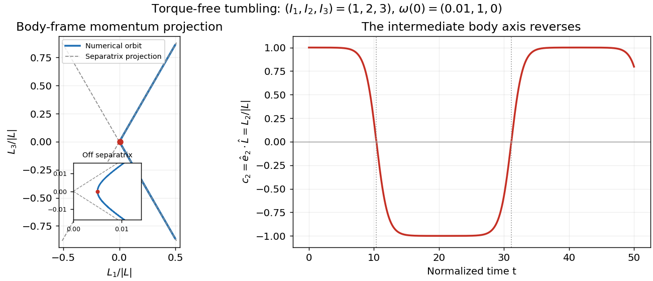
Torque-free reversals of a nearly aligned body axis
. Original independent Runge-Kutta method calculation in angular momentum and rotation matrix variables, starting with in the normalized intermediate-axis model. Left: body-frame orbit projected onto ; dashed lines are the intermediate-axis separatrix projections . The red point is the initial condition; the inset resolves its separation from those lines. Right: , with dotted lines at the first two zero crossings. The full angular momentum vector remains fixed in space. Details.
Both calculations use step size without rescaling either invariant. Over , the tumbling calculation changes rotational kinetic energy and squared angular momentum by less than relative to their initial values. Reconstructing in the fixed space frame gives relative error below . Halving the step changes the body components and rotation matrix entries by less than . These checks distinguish physical tumbling from numerical drift. On the exact intermediate-axis separatrix, approach to an intermediate-axis rotation takes infinite time; the recurrent off-separatrix example here is different.
Normalized intermediate-axis model 2026-10-14
Choose an inertia unit and an angular speed unit , so physical principal moments of inertia are , physical angular velocity is , and normalized time is . The Euler equations for a torque-free rigid body becomeThis is a physically admissible ideal planar mass distribution: is the perpendicular axis theorem. A book of finite thickness need not have these exact ratios.
For an original comparison, start with angular velocity , or , respectively. With , the transverse Euclidean norm stays small about axes one and three, but becomes order one about axis two. For the intermediate-axis start, its linearization givesThe hyperbolic functions contain a growing exponential function with rate . Reducing tenfold delays reaching the same small transverse amplitude by approximately normalized time units, once the growing term dominates. That delays the instability. Once the transverse angular velocity is comparable to the main component, the linearization ceases to describe the motion.
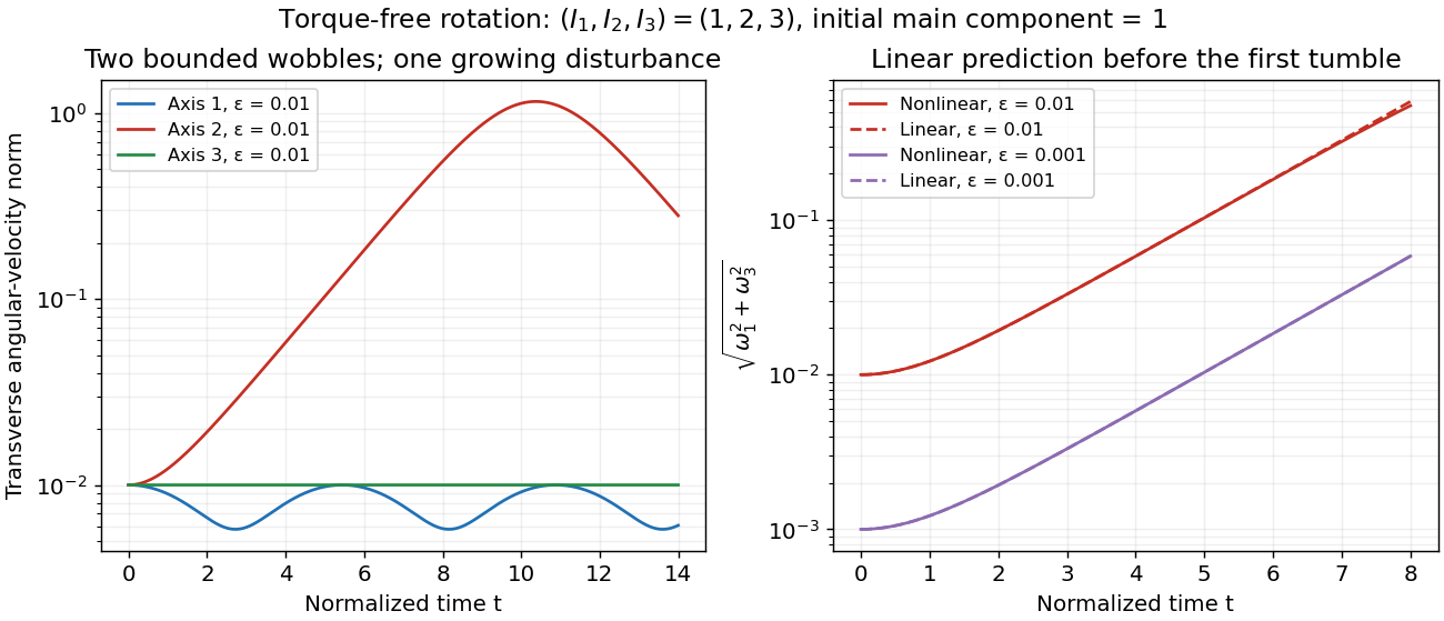
Small perturbations about the three principal axes
. Original Runge-Kutta method calculations for the normalized intermediate-axis model, with initial angular velocity , and . Left: transverse Euclidean norm relative to each initial principal axis. Right: full Euler equations for a torque-free rigid body compared with the displayed linearization, also using . Dashed curves are linear predictions. These are model curves, not measured throws. Details.
Markov interlacing lemma 2026-10-14
Differentiation preserves the ordering of interlacing roots of polynomials of equal or consecutive polynomial degrees. Iteration gives the result for every derivative for which both polynomials are nonconstant; common roots are allowed by a limiting argument. This is a result about the locations of roots of a polynomial, distinct from the Markov inequality for polynomial derivatives. Theorem A of Dimitar K. Dimitrov's account states the first-derivative result.
For a monic polynomial with distinct ordered real roots of a polynomial, each critical point lies between two consecutive roots by Rolle's theorem. Its logarithmic derivative gives . Implicit differentiation gives the displayed formula, so moving any root to the right moves every ordered critical point to the right, while the roots remain distinct. Iterating this statement for derivatives preserves componentwise ordering of their roots. Weak inequalities extend by continuity to repeated roots.
At a point in a normal orthonormal frame, torsion-freeness makes the frame brackets vanish there, hence the dual one-forms have zero exterior derivative there. Differentiating the interior product formula then leaves only , the divergence of a Riemannian vector field. Since the point is arbitrary, the identity holds globally.
Caplet 2026-10-14
One payment period of an interest-rate cap. For , its value at the reset date is . Thus the caplet is equivalent before reset to units of a put expiring at on the maturity- zero-coupon bond, with strike .
Two-factor interaction 2026-10-14
A two-factor interaction means that changing one factor has a different effect at different levels of another. For a two-level factorial design, its sign column is , and four times its coefficient is the corresponding difference of differences. It can be confounded with other factorial contrasts in a fractional factorial design.
For the differential one-form , a nonzero integrating factor makes an exact differential form locally. If it equals , then , , and equality of mixed partial derivatives gives the displayed compatibility condition. Conversely this condition is local sufficiency for smooth coefficients on a small rectangle; global exactness additionally depends on the domain. Zeros of the multiplying factor can change the solution set, so equivalence is asserted only where the factor is nonzero.
For with continuous , the integrating factor gives the displayed solution. It is continuous at the step and solves the differential equation classically on each side; the derivative jumps by one. The value assigned to the Heaviside step function at the single point zero does not affect the integral. A discontinuity in would instead produce an unintended delta term in its distributional derivative.
Trigonometric integral 2026-10-14
The sine and cosine integrals accumulate and , with different normalizations at zero and infinity. They arise in oscillatory integrals, Fourier transforms of singular kernels and Fourier series of logarithmic profiles.
The integral remainder in Taylor theorem for gives the exact finite identityFor , , so the nonnegative remainder is at most and tends to zero. At it is at most , proving both convergence to and an explicit error bound without assuming the logarithmic power series beforehand.
For any algebraic field extension , including an infinite one, its ring of elements integral over is an integral extension of . The Lying-over theorem, going-up theorem and incomparability theorem for integral extensions give . The argument does not require that be Noetherian or finitely generated over .
Volume average 2026-10-14
A volume average is the normalized integral average of a field over a three-dimensional region of finite positive volume. For a fixed region, differentiating in time commutes with this average under the usual regularity conditions. The divergence theorem converts the average of a divergence into its net boundary flux divided by volume.
There are unlisted articles, also show them or only show them.