
Use SI units throughout: , , and . The effective propagation distance is , givingIn the supplied Cornu spiral, the endpoint at is approximately . HenceMore accurate Fresnel integrals, and , give . The central light intensity is increased to about times the unobscured value, an increase of roughly .
There is no violation of conservation of energy: the aperture reduces the total transmitted power, while removing contributions that partly cancel the central field redistributes the transmitted power across the observation plane. In particular, the square aperture does not give the same central field as a circular aperture of a superficially similar size.
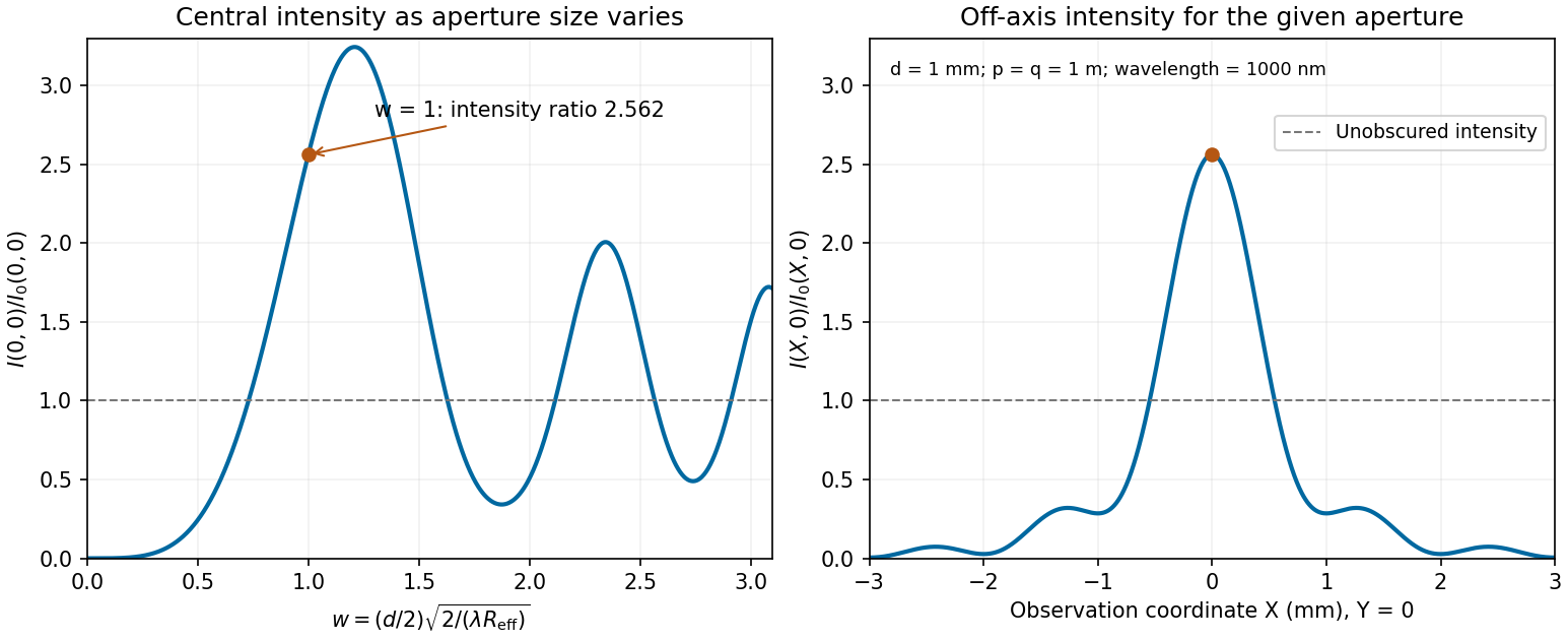
Calculated central intensity and an off-axis section for the square aperture in the Fresnel approximation
. Details. 
Write and for the axial source and observation distances, and put . The aperture is . Under the Fresnel diffraction, the spherical incident wave amplitude is effectively constant over this small aperture, while its quadratic wave phase must be retained. Therefore the two transverse integrals separate:where contains the source strength, the propagation distances and a common phase factor.
Use the dimensionless variable and define the optical normalization of Fresnel integralsThe oddness of makes the bracket , soThis square-aperture Fresnel diffraction normalization is especially useful for comparing with no aperture. In the same Fresnel diffraction, the unrestricted one-dimensional Fresnel integral is ; its square is . Thus, writing for the unobscured field at the same point,The normalization has the correct no-aperture limit because in this convention.
The expression is a scalar diffraction theory integral for a monochromatic wave. The complex quantity represents a field complex amplitude, with physical field obtained by taking the real part after multiplication by . The light intensity is proportional to . The coordinates label transverse positions in the aperture plane, is its transmitting region, and is the incident field multiplied by the aperture's complex transmission. The wavenumber is in the propagation medium, and is the axial propagation distance if already includes the incident field.
To derive the Fresnel diffraction, start from Huygens-Fresnel principle contributions with propagation factor . With the coordinate origin at the projection of into the aperture plane,The paraxial approximation requires , where . Replace the slowly varying and the obliquity factor by their axial values, but retain the quadratic variation of wave phase. Neglect of the next wave phase term requires over the relevant aperture. Thus, apart from a common constant,The quadratic wave phase may be of order one or much larger; setting it to zero would require the stronger conditions for Fraunhofer diffraction. The scalar treatment also neglects the detailed vector field at aperture edges and assumes dimensions large enough compared with wavelength for this approximation to be useful.
For a finite-distance axial point source at distance and an observer at distance , the incident field contributes its own quadratic wave phase. If instead denotes only the aperture transmission, the combined curvature is described by an effective distanceThese are two equivalent conventions for distributing the incident wave phase between and the exponential. Both distances must be included in the later calculation.
Put . Eliminating the middle-segment complex amplitudes using the right-hand boundary conditions givesHence the displacement reflection coefficient isFor finite positive real mechanical impedances, its denominator cannot vanish at real . The real and imaginary parts of the numerator must therefore vanish separately:This gives all three possibilities.
If the exterior strings differ, , then , so andThe middle segment is a quarter-wave impedance transformer. Its two reflected contributions cancel at these odd quarter-wavelength thicknesses. Here is specifically the wavelength in the middle string; the matching is not generally valid at every frequency.
If but differs, the second condition requires , givingA whole number of half-wavelengths reproduces the exterior mechanical impedance at the input. The formal limit is zero frequency or zero segment length, rather than a finite-wavelength resonance.
Finally, if , both conditions hold identically: . Since the system is lossless, each of these cases also gives unit transmitted power.
Let the middle segment occupy . Normalize the incident displacement complex amplitude to one, suppress the common time factor , and chooseHere is the reflected complex amplitude at , and are the rightgoing and leftgoing middle-segment complex amplitudes referenced to , and is the outgoing complex amplitude referenced to . The middle wavenumber is , andis the propagation phase factor across the lossless middle segment.
At each junction, continuity of displacement and transverse force means continuity of and . Using givesThese boundary conditions also include all multiple reflections inside the middle segment: and are the total travelling components, not just the first waves to cross a junction.
The instantaneous rightward energy flux along a string is the transverse force times the transverse velocity,For a rightgoing time-harmonic wave of peak displacement wave amplitude , averaging over a wave period givesA leftgoing time-harmonic wave has the opposite signed energy flux. The positive ratios of reflected and transmitted power to incident power are thereforeAll explicit angular frequency factors cancel. In the ideal wave equation on a string, and the two linear mass densities are constant, so the mechanical impedances have no frequency or wavelength dependence. Consequently is independent of wavelength even though the two string wavelengths generally differ.
Finally,This is conservation of energy at a lossless, massless junction. The transmitted displacement wave amplitude can exceed the incident one when ; the factor is essential when comparing power.
Place the junction at and use the complex amplitude convention . With incident displacement wave amplitude , writeHere and are displacement wave reflection and transmission coefficients, and . The junction is assumed massless, with no externally applied transverse force, and both strings have the common equilibrium tension . Continuity of displacement and transverse force givesSince , these become and . Solving,A larger right-hand mechanical impedance produces a reflected displacement with reversed sign, as expected in the fixed-end limit . Equal mechanical impedances give and .
Use transverse displacement , small slopes and constant tension . For a short string element of length , Newton's second law gives . Hence the wave equation on a string iswhere is the linear mass density, in .
The mechanical impedance of a rightgoing travelling wave is the transverse driving force divided by the transverse velocity at the driven section. Choose the force exerted by the material to the left on the material to the right, . For , the transverse velocity is . Thus the positive characteristic impedance of a stretched string isA leftgoing component has with this fixed orientation of force. Specifying the orientation avoids confusing that propagation sign with a negative material mechanical impedance.
A chi-squared test compares the sum of squared standardized regression residuals with the appropriate chi-squared distribution. With both line parameters fitted, the data give on degrees of freedom, with upper-tail P-value about : the fitted exponential decay model describes the data adequately.
First consider fixing the alternative lifetime at its central value . Its slope is . One must refit the normalization rather than retain the earlier intercept. Minimization over the intercept gives , andon degrees of freedom, with upper-tail P-value about . Thus that fixed central lifetime gives a substantially worse fit than . Equivalently, the increase after profiling over the intercept isThis fixed-value comparison does not yet include the uncertainty of the alternative measurement.
For the compatibility of independent lifetime measurements, include both errors. Under the approximately Gaussian lifetime-error model, equality of the two true lifetimes is tested byThis has one degree of freedom and P-value approximately , equivalent to a -standard deviation discrepancy. The two measurements are therefore in mild tension: equality is rejected at a significance threshold, but not at . There is no unique yes-or-no compatibility verdict without choosing such a threshold. Treating the alternative central value as exact would overstate the disagreement between the experiments.
The lifetime that provides the best fit to these six rates remains , not . The compatibility calculation above assumes the two experiments have independent uncertainties; a shared systematic error would require its covariance.
For an independent count with a Poisson distribution, collected for exposure at rate , the expected count is and its standard deviation is . The fractional rate uncertainty is consequentlyA target of requires counts at each proper-time setting. The exposure time for a Poisson rate at fixed fractional precision is therefore , givingSince the settings are acquired independently rather than simultaneously,Nearly three quarters of the exposure is spent at the latest, lowest-rate setting. Proper time in picoseconds labels the decay distribution; it is not the laboratory acquisition time in days. This estimate assumes counting statistics dominate, with no additional background-subtraction uncertainty or acquisition overhead.
Assume independent approximately Gaussian log-rate errors with known common standard deviation . The weighted least squares objective isSince all weights agree, the normal equations for linear least squares reduce toFor these data, , , and . Hence and .
The covariance matrix of the fitted slope and intercept follows from the inverse weighted design matrix product, or directly by writing both estimates as linear combinations of the independent :This givesThe parameter conversion and first-order propagation of uncertainty areConsequently,These are one-standard deviation errors. The estimates are correlated, since . The minimum is for four residual degrees of freedom. Because is supplied as a known measurement uncertainty, it should not be rescaled by the observed reduced . This is a log-linear exponential-decay fit.
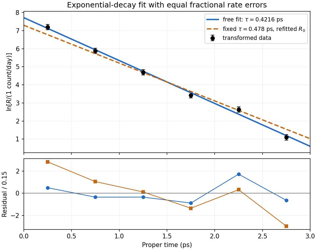
Log-rate fit and the effect of imposing the alternative lifetime
. Original calculation from the exam measurements. The solid line fits both lifetime and normalization; the dashed line fixes and refits its normalization. The lower panel shows standardized log-rate residuals for the two fits. No error bar is assigned to proper time. Details.
Use in picoseconds and . Since the time uncertainty is negligible, only the vertical errors enter. First-order propagation of uncertainty givesThe transformed measurements areThus the logarithmic transformation converts constant fractional rate uncertainties into approximately equal absolute log-rate uncertainties. The equality is the linear error approximation; finite error bars would become slightly asymmetric under an exact logarithm.
Take the natural logarithm of the exponential decay model. To keep the logarithm dimensionless, choose the reference rate and defineThen . With time measured in picoseconds, the slope has units and the intercept is dimensionless. A straight-line linear regression in these variables therefore estimates the inverse mean lifetime and logarithmic normalization.
Each energy eigenstate picks up its own phase under unitary time evolution. The relative phase therefore changes at . After removing an irrelevant global phase, the state isThe diagonal position matrix elements vanish, but the annihilation operator and creation operator giveThe two off-diagonal cross terms in the expectation value yieldThus the angular frequency is , and the magnitude of the oscillation, meaning its amplitude, isThe peak-to-peak displacement is . The phase fixes where the oscillation starts but does not change . A pure or preparation has no mean oscillation, whereas an equal-weight quantum superposition maximizes its amplitude within this two-state family. The motion is produced by interference between energy eigenstates, rather than by a changing occupation of either one.
The standard deviations defining the position and momentum uncertainties satisfy and . Part (a) makes both means zero. Using the second moments from part (b),Multiplication givesThe Heisenberg uncertainty relation requires only . Among the oscillator energy eigenstates, equality occurs solely for the ground state ; the excited states have larger uncertainty products.
For the harmonic-oscillator number-state second moments, the number operator gives , while the canonical commutation relation gives . Terms with or have zero diagonal matrix elements, since they change the occupation number by two. ThereforeConsequently the potential energy and kinetic energy means areTheir sum is the oscillator energy eigenvalue . Their equality is also the virial theorem result for a quadratic potential, here derived directly from the ladder operators.
Write and . Inverting the annihilation operator and creation operator definitions givesThe ladder operators take to orthogonal quantum harmonic oscillator energy eigenstates and . Thus , andFor , the lowering term is simply zero. The conclusion concerns an individual energy eigenstate; interference between different eigenstates can produce nonzero expectation values.
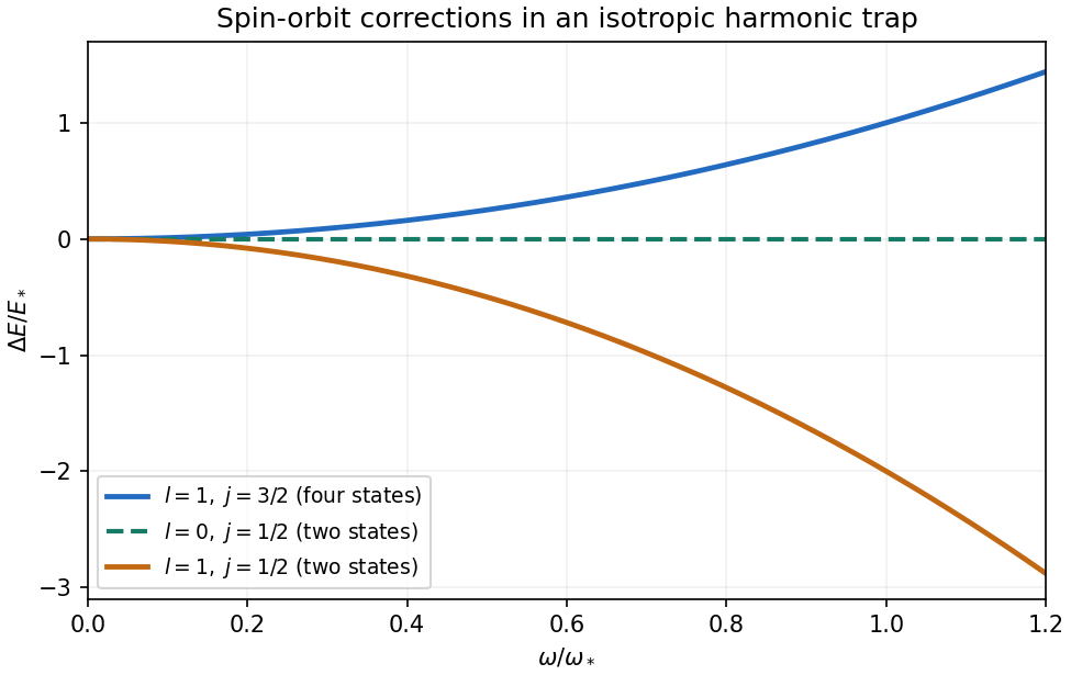
For the isotropic three-dimensional quantum harmonic oscillator, , hence is constant. No radial integral remains, so the spin-orbit energy shift in a central potential reduces toFor , the only possibility is , and the bracket vanishes. For , coupling to spin one-half permits and , whose brackets are and . ThusThese spin-orbit shifts of an isotropic harmonic oscillator are a zero line, a downward parabola, and an upward parabola of half the downward magnitude. They are independent of the radial excitation number, and their magnetic multiplicities are respectively two, two and four. Their weighted mean within the manifold is zero: .

The attractive Coulomb potential energy is , soUse precisely the radial normalization stated in the PDF: the radial probability measure is . The supplied function hasIts integral is one, since . In particular,This calculation uses the supplied convention, rather than multiplying a separately normalized standard radial function by an extra .
The addition of angular momentum bracket is . Substitution in the spin-orbit energy shift in a central potential therefore givesHere is the supplied Bohr radius. The negative sign means the member of the pair is shifted downward by this spin-orbit interaction; it is not the total hydrogen binding energy.
The total angular momentum operator is . Since orbital and spin operators act on different factors of the tensor product, they commute, and expanding givesA coupled angular momentum eigenstate is a simultaneous eigenstate of these three squared operators, with eigenvalues , and . Thus the angular factor in the spin-orbit interaction is the numberThe other factor, , is radial. It commutes with the angular operators, and a central-potential energy eigenstate separates into a radial wavefunction and an angular spinor. Taking its radial expectation value therefore givesThis spin-orbit energy shift in a central potential is independent of , so rotational symmetry preserves the magnetic degeneracy within a fixed multiplet. It is a first-order fine structure correction; the given coefficient already includes the relativistic factor needed for the electron's spin-orbit coupling.
There are unlisted articles, also show them or only show them.