
The convolution of two aperture functions in one dimension isWith Fourier transform convention , the convolution theorem statesThe first identity follows by substituting the convolution integral, putting , and separating the resulting double integral into times . For an absolutely integrable pair the interchange is justified by absolute convergence; finite optical apertures satisfy suitable integrability assumptions.
In Fraunhofer diffraction, the observed field is the Fourier transform of the transmitted complex aperture field. For two identical slits, let be one slit and use a pair of Dirac delta distributions to locate the centres:Consequently . For a rectangular slit, , giving a single-slit diffraction envelope times the double-slit interference factor in intensity. A phase reversal replaces the plus between the deltas by a minus, giving instead, as in B7.
More generally, an -slit array is a single-aperture function convolved with a finite comb. Its field contains the factorThis separates the narrow diffraction grating maxima from the individual-aperture envelope. The same reasoning holds in two transverse dimensions. Multiplying an existing aperture by an additional finite mask instead convolves their field transforms and can broaden features. These are operations on complex fields: intensity is the squared modulus of the final field and cannot generally be substituted into the field-level convolution theorem.
Past exam of the physics A course of the University of Cambridge 2018 Paper 2 Section C C11 d Solution Created 2026-10-18 Updated 2026-10-20
In a normal metal, the electrical resistivity can often be approximated using Matthiessen's rule,Static impurities, defects and grain boundaries scatter conduction electrons even as , giving the residual resistivity. Thermal lattice phonons add a temperature-dependent contribution through electron-phonon scattering. In a clean three-dimensional acoustic model, small-angle electron-phonon transport at low temperature gives at low ; once thermal phonon populations are approximately classical, the resistivity is approximately linear in . An electron-electron contribution proportional to can be relevant in some low-temperature ranges.
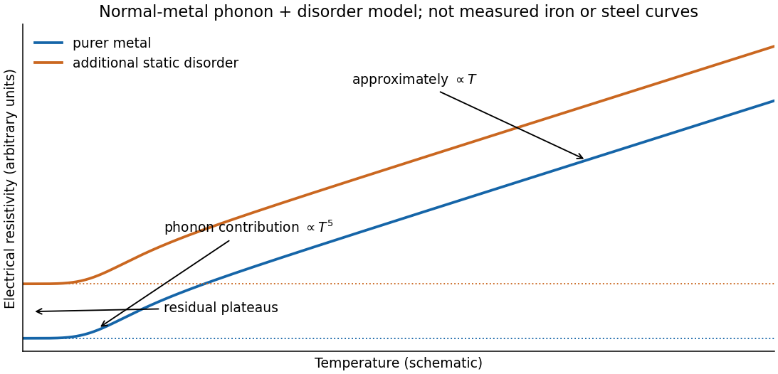
Schematic normal-metal resistivity with residual, low-temperature phonon and approximately linear high-temperature regimes
. Details. Carbon in mild steel, together with associated disorder, strain and microstructural changes, adds scattering and generally raises the residual resistivity relative to purer iron. Thus a dilute alloy may have a similar broad phonon-dependent rise but a larger baseline. The sketch is a generic phonon-plus-disorder model, not measured iron data. Iron's magnetic scattering and phase changes, and real steel's phases and processing history, can add structure; the simple sum is approximate rather than an exact material law. The expected explanation is greater electron scattering from the added carbon and resulting disorder.
Past exam of the physics A course of the University of Cambridge 2018 Paper 2 Section C C11 c Solution Created 2026-10-18 Updated 2026-10-20
Interpret “3 mm wire” as a circular wire of diameter , and take the current density as uniform. One conduction electron per atom givesUsing , the drift velocity corresponding to a current magnitude of isIt points opposite to conventional electric current. A simple distance scale over the cycle is , but this treats the magnitude as constant. For sinusoidal mains, alternating-current drift excursion gives zero net displacement after a full cycle.
If is the usual root mean square current, and the displacement amplitude and total absolute drift distance per cycle areIf instead denotes peak current, these become and . The paper does not state peak versus RMS; the characteristic drift is the boxed on whichever current convention is chosen. It also does not explicitly say diameter; taking as the radius would reduce all these velocities and drift distances by four. None of these distances is the microscopic path travelled at roughly the Fermi velocity between scattering events; that path cannot be obtained from the supplied current alone.
Past exam of the physics A course of the University of Cambridge 2018 Paper 2 Section C C11 b Solution Created 2026-10-18 Updated 2026-10-20
Let denote the elementary charge, so an electron's charge is . In the relaxation-time Drude model with positive transport effective mass,The steady drift velocity is , defining positive electron mobility . The current density is opposite to the electron drift:By the definition of electrical conductivity, , soIts units are . The mobility definition alone establishes the result in the scalar linear-response regime; the relaxation-time equation supplies a microscopic approximation for .
Past exam of the physics A course of the University of Cambridge 2018 Paper 2 Section C C11 a Solution Created 2026-10-18 Updated 2026-10-20
A Bloch state in a crystal experiences a periodic lattice potential. Its band dispersion relation encodes the lattice response, so an effective mass allows a wavepacket's acceleration under a weak applied force to be described without explicitly following the microscopic periodic forces.
In one dimension the wavepacket group velocity and semiclassical equation for crystal momentum areDifferentiating the first equation with respect to time givesDefining yieldsThis band effective mass is controlled by band curvature, not the slope. A band minimum has positive ; a band maximum has negative electron and is often more conveniently described with positive-mass electron holes. In three dimensions the inverse effective mass is generally a tensor, . The scalar formula assumes motion along a specified direction in an isolated band, weak fields and negligible interband transitions; the bare electron mass has not physically changed.
Past exam of the physics A course of the University of Cambridge 2018 Paper 2 Section C C10 e Solution Created 2026-10-18 Updated 2026-10-20
Assume sodium supplies one conduction electron per atom. The supplied Fermi energy givesThe gas is strongly degenerate at room temperature. For one mole, and . Using the requested estimate,The supplied mass density determines the answer per unit volume: . ThereforeThe density is not needed for the molar heat capacity once is supplied. Using the precise Sommerfeld expansion coefficient instead gives .
Either electronic estimate is only about of the stated measured total. Most of the total heat capacity comes from lattice phonons, whose high-temperature Dulong-Petit law limit is . The remaining difference from need not be electronic: anharmonic lattice effects and the difference between heat capacity at constant pressure and heat capacity at constant volume also contribute. The paper does not specify the measurement constraint, so the two totals should not be equated exactly.
Only a shell of energy width of order near the Fermi energy can change occupation: much lower states are blocked by the Pauli exclusion principle. The thermal-shell estimate of electronic heat capacity countsTo recover the rough coefficient requested in the paper, assign each of these active particles an excitation energy of order . ThenThe differentiation matters: the active shell itself widens as temperature rises. This argument explains the small linear-in- electronic heat capacity; its shell width and average excitation energy are heuristic, so it does not establish a precise numerical prefactor.
A controlled calculation from the Fermi-Dirac distribution gives a nearby but different result. At fixed particle number, the Sommerfeld expansion yieldsThus is a rough estimate of the exact free-electron coefficient , not an exact consequence of the stated density of states. Both require .
The occupation probability of an individual one-electron state is the Fermi-Dirac distribution,At , it is a step: one below and zero above it. Heating rounds the step over an energy range of order a few , creating empty states below and occupied states above the chemical potential. At every positive temperature, .
For fixed in the three-dimensional free electron model, the chemical potential is determined by ; it is not exactly constant. In the degenerate regime , the Sommerfeld expansion givesIt is therefore reasonable in a simple low-temperature sketch to set , provided this approximation is stated. The figure includes the leading small shift. At much higher temperature the fixed- approximation fails and the distribution approaches the classical dilute limit. The plotted occupation is , rather than the energy distribution .
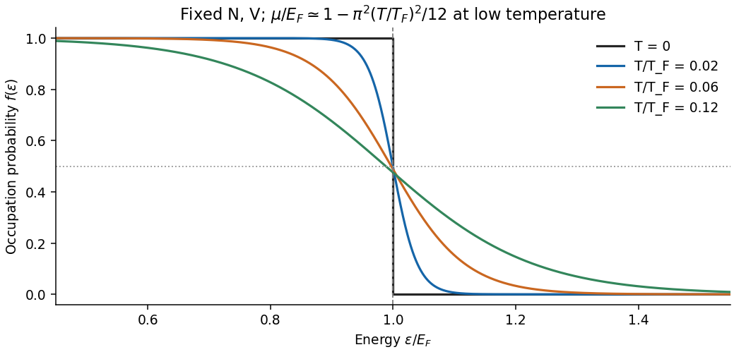
Thermal rounding of Fermi-Dirac occupations at fixed particle number, with the leading chemical-potential shift
. Details. Impose periodic boundary conditions on a large cubic box. The allowed wavevectors occupy a lattice of cell volume in wavevector space. Including the two spin states, the number of states with magnitude at most isUsing and differentiating gives the total, spin-summed three-dimensional free-electron density of states,It counts states per unit energy; divide by for states per unit volume per unit energy. At zero temperature, the Fermi-Dirac distribution fills all states up to the Fermi energy, givingWriting givesThe energy zero is the bottom of the free-electron band. The electron Fermi temperature is .
Past exam of the physics A course of the University of Cambridge 2018 Paper 2 Section C C10 a Solution Created 2026-10-18 Updated 2026-10-20
Use the quantum free electron model: conduction electrons move as independent particles in a three-dimensional box of volume , with a uniform positive background replacing the ionic lattice potential. Neglect the detailed periodic potential and explicit electron-electron interactions; the interior one-electron dispersion relation is . The boundary confines the particles, and its detailed shape does not affect the bulk state count in a sufficiently large sample.
The electrons are spin- fermions: each spatial quantum state accommodates two opposite spin states, with occupations given by the Fermi-Dirac distribution and the Pauli exclusion principle. A fixed number of conduction electrons and thermal equilibrium are assumed. Collisions can be represented by a phenomenological momentum relaxation time for transport, but are unnecessary for the equilibrium state counting here. These assumptions distinguish the quantum model from a classical Maxwell-Boltzmann electron gas.
At an ordinary point or a massless join, the string is continuous, soWith no concentrated transverse force or point mass, transverse force balance requiresFor the common tension in this problem, the slope is therefore continuous as well. A jump in linear mass density changes wave speed, but introduces no finite inertial force at a zero-length join. A point mass, external support force, or unequal tensions would require modified boundary conditions.
For a rightgoing harmonic travelling wave in the lossless string, its force and transverse-velocity complex amplitudes satisfy with real . Thus the supplied mean-power expression giveswhere is the displacement complex amplitude and for convention . The same result follows directly from instantaneous string power averaged over a cycle. The amplitudes here are peak amplitudes; with root mean square force or velocity the factor is absent. If reflections return to the driver, its net mean input is still , but its input mechanical impedance need not equal the travelling-wave value .
A characteristic wave impedance relates an effort-like quantity to its conjugate flow-like quantity in a single travelling wave: for a mechanical wave these are force and velocity, and their product is power. The sign depends on the propagation and force conventions. Use the transverse force transmitted towards increasing , . A rightgoing travelling wave has transverse velocity , soThis is the positive characteristic impedance of a stretched string. A leftgoing component has with the same force orientation. Its units differ from pressure-based acoustic impedance because it uses force, rather than force per area.
The symbol here is linear mass density, with units . A short element has transverse forcebecause small slopes give . Its mass is . Applying Newton's second law, dividing by , and taking the limit gives the wave equation on a string,The derivation assumes constant positive tension, small transverse displacements and slopes, a flexible string with negligible bending stiffness, and negligible damping. Variations of tension due to the motion enter beyond the linear approximation.
For mutually incoherent spectral components, the detected intensities add. If describes the mean output spectral intensity, the interferogram isSubtract the constant background, scan the mirror with a calibrated displacement, and take the Fourier transform with respect to delay . This is Fourier transform spectroscopy. The transform recovers the spectrum subject to detector response, finite scan length and any window function. Sampling the displacement finely enough to resolve the shortest optical fringes avoids aliasing.
Using the usual reciprocal-maximum-delay resolution estimate, , and , givesThe mirror displacement is measured from zero optical path difference. This delay-range resolution in Fourier transform spectroscopy is a conventional estimate: a specified window and resolution definition introduce a numerical factor. For example, a symmetric rectangular delay window has its first instrumental zero at , which would give under that particular criterion. The paper does not specify a line-profile criterion; the standard estimate states its convention explicitly.
The two sodium lines are distinct optical frequencies, so their rapidly oscillating mutual cross terms average to zero at the detector. Assuming equal line strengths and negligible individual linewidths, add their separate interferograms. Write and . With the total mean output intensity,For mirror displacement this becomesThis is spectral doublet from Michelson visibility revivals. Since , . Numerically,The first interference visibility zero occurs at , with further zeros at odd multiples of that distance. Visibility is restored at integer multiples of . The signed envelope has period : alternate high-visibility packets have opposite fringe phase. Unequal line strengths leave a nonzero minimum visibility, and finite linewidths introduce a further decaying envelope; the wavelength data alone specify neither effect.
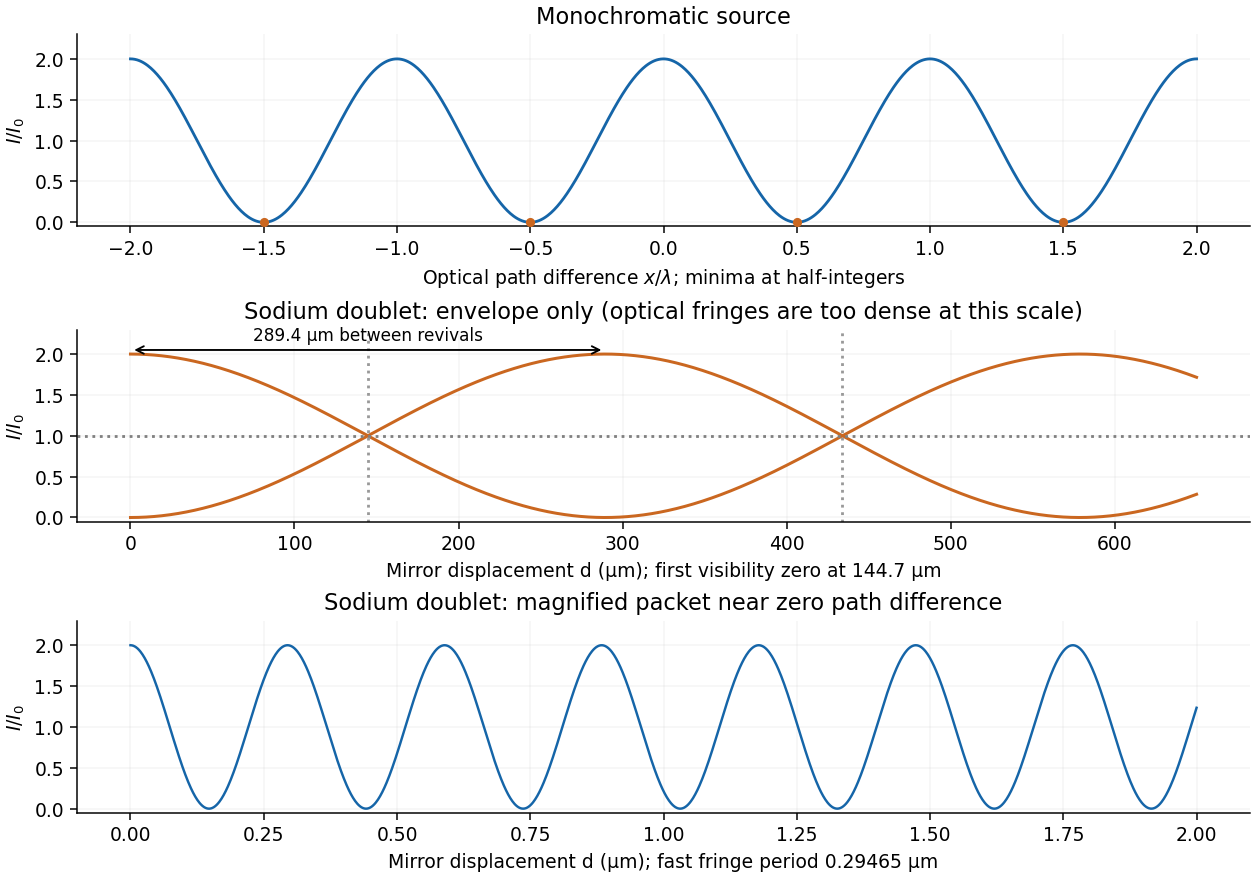


Take the two interfering complex amplitudes to have equal intensities and relative phase . The interference cross term then givesThus the mean intensity is , the maximum is , and the minima areThe optical path difference period is and the mirror-displacement period is . The assumed equal intensities refer to the two fields at the chosen output, with matching polarization of waves and full optical coherence. They set the normalization; they should not additionally be interpreted as all incident light entering that output port. A physical lossless Michelson interferometer has a complementary second output.
There are unlisted articles, also show them or only show them.