
Past exam of the physics A course of the University of Cambridge 2019 Paper 2 Section D D13 c Solution Created 2026-10-18 Updated 2026-10-20
In a metal, mobile electrons transport heat as well as electric charge. A temperature gradient creates an imbalance between carriers arriving from warmer and colder regions. The resulting heat current obeys Fourier's law for an isotropic material, where thermal conductivity has units . For a bar of area carrying steady heat flow , when parasitic losses are negligible.
A kinetic estimate for the electronic contribution iswhere is the electronic heat capacity per volume, the Fermi velocity, and the heat-transport mean free path. Fermi-Dirac statistics and the Pauli exclusion principle restrict thermal rearrangements to states near the Fermi surface, rather than allowing every electron to contribute a classical heat capacity. A degenerate parabolic band givesUsing the Drude model form for electrical transport, the relation between thermal and electrical relaxation times in metals becomesFor scattering that relaxes heat and charge currents similarly, and the Wiedemann-Franz law follows:Thus good electrical conductors are usually good thermal conductors. The correct quantum Lorenz number differs from a naive classical electron-gas estimate.
Scattering from impurities, boundaries and phonons limits the heat-transport path. In an impurity-dominated low-temperature regime with approximately constant relaxation time, is approximately proportional to . Where phonon-limited electrical resistivity is proportional to and the Wiedemann-Franz approximation is applicable, can be roughly temperature independent. Inelastic processes can relax heat and charge currents differently, so the Lorenz ratio is not universal at all temperatures. Lattice phonons add a separate positive thermal contribution; the measured total is , and the electronic Wiedemann-Franz expression should not be applied blindly to that total.
Past exam of the physics A course of the University of Cambridge 2019 Paper 2 Section D D13 b Solution Created 2026-10-18 Updated 2026-10-20
Semiconductor doping introduces controlled impurities to alter equilibrium carrier populations and electrical conductivity. In an intrinsic semiconductor, thermally excited electrons in the conduction band and electron holes in the valence band have equal densities . A shallow donor impurity, such as phosphorus in silicon, supplies an electron from an impurity level just below the conduction-band edge. Once ionized it is positively charged, and the material is n type. An acceptor impurity, such as boron in silicon, accepts a valence electron into a level just above the valence-band edge, leaving a mobile hole and a negatively charged ionized impurity; the material is p type.
With dopant densities , charge neutrality requiresFor fully ionized, nondegenerate dopants at equilibrium, the semiconductor mass-action law gives . In a substantially n-type sample, , soThe corresponding p-type result is and . The majority population grows while the minority population decreases; adding donors does not simply add equal numbers of free electrons and holes.
The Fermi energy shifts toward the conduction band for n-type material and toward the valence band for p-type material. In the nondegenerate approximation,where are effective band-edge state densities. At very low temperature, dopants may not be ionized and carrier freeze-out occurs. At intermediate temperatures, ionized dopants dominate the carrier density; at sufficiently high temperature, intrinsic excitation can dominate. Heavy doping can produce degenerate carrier statistics, invalidating these Boltzmann expressions.
The electrical conductivity is . Doping usually raises the majority carrier density, but ionized impurity scattering can lower mobility, so conductivity need not scale indefinitely with dopant concentration. Joining p-type and n-type regions creates a p-n junction, with a depletion region and built-in electric field established by carrier diffusion and compensating drift. The fixed ionized dopants, not an absence of all charge, account for the depleted region's net charge density.
Past exam of the physics A course of the University of Cambridge 2019 Paper 2 Section D D13 a Solution Created 2026-10-18 Updated 2026-10-20
The Hall effect is a transverse electric response to a magnetic force on moving charge carriers. Take conventional current density and magnetic field in a conducting slab. For one carrier type of number density and signed electric charge , the drift velocity is . Carriers initially deflect sideways until a Hall electric field balances the magnetic Lorentz force:The Hall coefficient is thereforeFor electrons it is , whereas a simple hole-dominated conductor gives . The sign reveals the effective carrier sign; the magnitude estimates their density in the one-carrier approximation.
For width along and thickness along , . Define the signed Hall voltage by , namely the electric potential at the lower- edge minus that at the higher- edge. ThenThis explicit contact convention fixes the voltage sign. A Hall bar with longitudinal and transverse contacts measures both electrical resistivity and the Hall response. Reverse the field and take the part of the transverse voltage odd in to suppress longitudinal-voltage pickup from misaligned contacts; reversing current provides another useful check.
A Hall measurement is useful for carrier identification, semiconductor doping measurements and magnetic-field sensing. Combining a one-carrier with electrical conductivity gives a mobility magnitude . However, mixed electron and hole conduction is not described by a single density: in weak fields,The response weights mobilities differently from ordinary conductivity. Complicated energy bands, anisotropic Fermi surfaces and multiple bands can likewise change the simple interpretation in metals; a positive Hall coefficient does not mean that the material contains positively charged fundamental electrons.
Past exam of the physics A course of the University of Cambridge 2019 Paper 2 Section C C11 d Solution Created 2026-10-18 Updated 2026-10-20
With length measured in units of , plot the real functionOnly the portions with can equal , so the strip between the horizontal lines and identifies allowed energy bands. The band edges of a repulsive delta-comb potential have the following approximate first intervals:Each interval corresponds to energy ; the intervening intervals are forbidden. The exact upper endpoints follow from . The lower endpoints solve inside . The divergence suggested by at the origin is removable, and , so there is no zero-energy state in the repulsive model.
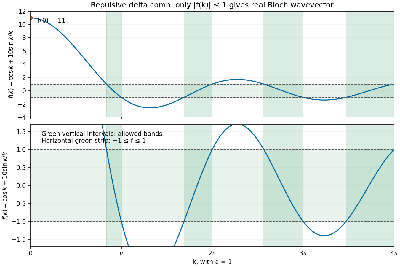
Calculated delta-comb discriminant for barrier strength 10, with allowed bands marked by the strip between minus one and plus one
. Details. The periodic barriers produce separated energy bands and band gaps, unlike the continuous free-particle spectrum. A finite -atom loop has discrete states within these bands. Whether the material conducts still depends on band filling: one electron per primitive cell half-fills a spin-degenerate band, while two electrons per cell can fill the first band and place the Fermi energy in a gap. Band gaps alone do not establish that every filling is insulating. At high , the perturbing term becomes relatively small and the spectrum approaches free-electron behaviour in relative terms.
Between delta barriers, and the Schrödinger equation gives , with for positive energy. Write the state and derivative as a two-component vector . Free propagation across one interval of length isThe wavefunction is continuous at a delta barrier, while its derivative jumps by , with . Thus the barrier matrix isBloch's theorem requires . Both and have determinant one, so the two eigenvalues of are and . Taking its trace givesTherefore the Floquet discriminant of the delta-comb Kronig-Penney model yieldsThis trace argument is the one-cell transfer method for the Kronig-Penney model. The loop imposes the additional discrete values of derived in part (b). Real requires the right-hand side to lie in , giving allowed energy bands; values outside this range are band gaps. The strength has units of energy times length, because a Dirac delta distribution has units of inverse length.
A Bloch state on the loop has , with . Its circumference is , so . Single-valuedness after one complete circuit requires the periodic boundary conditionThereforeThe allowed Bloch wavevectors are spaced by . Values of differing by label the same crystal momentum modulo a reciprocal lattice vector, so there are inequivalent choices in one Brillouin zone. In this notation is the Bloch wavenumber, not a dimensionless phase; is dimensionless. Spin gives additional states but does not alter this condition.
Past exam of the physics A course of the University of Cambridge 2019 Paper 2 Section C C11 a Solution Created 2026-10-18 Updated 2026-10-20
The quantum free electron model treats conduction electrons as independent particles moving in an approximately constant potential, with parabolic dispersion relation . Fermi-Dirac statistics successfully explains important features such as a Fermi energy and a small electronic heat capacity, but a constant potential gives no band gaps and cannot by itself explain why different band fillings produce metals, semiconductors and band insulators. It also misses lattice-dependent effective masses, detailed directional responses and the topology of real Fermi surfaces. Scattering and finite electrical resistivity require additional physics.
The nearly-free electron model introduces a weak periodic lattice potential. Bloch's theorem replaces individual free plane waves by Bloch states, and Fourier components of the potential mix plane waves whose wavevectors differ by a reciprocal lattice vector. Near degeneracy at a Brillouin zone boundary, this coupling opens a band gap; for a two-wave crossing its size is . Away from the crossing, energies remain close to free-particle values. Band curvature produces band effective masses, and band filling determines whether the Fermi energy lies inside an allowed band or a gap.
The improvement is the inclusion of lattice periodicity, rather than a switch from classical to quantum statistics: the quantum free electron model already uses Fermi-Dirac statistics. The strong delta barriers in the later numerical example are treated exactly by the Kronig-Penney model, rather than by assuming that their strength is perturbatively small.
Use temperature-dependent X-ray diffraction, with the crystal in a controlled heating stage and a detector measuring diffracted directions. A reflection occurs when the scattering wavevector matches a reciprocal lattice vector, or equivalently when Bragg's law is satisfied. Record peak positions and intensities while heating to infer changes in lattice spacings and structure.
A monatomic conventional BCC cell has nonzero crystal basis structure factor only when is even. For FCC the indices must be all even or all odd. The change in reflection selection and peak positions therefore distinguishes the phases. For instance, BCC starts with a family whereas FCC starts with , when indexed in their own conventional cells.
The transformation can create multiple orientation variants, grains, strain and phase coexistence. A reciprocal point that formerly satisfied the diffraction geometry may disappear or move off a fixed detector; a loss of one spot alone does not identify the new phase. Thermal expansion shifts peaks, thermal motion weakens coherent intensities, and hot iron may oxidize without a protective atmosphere.
After transformation, scan crystal angle and scattering angle or use an area detector to locate the new reflections. If single-crystal order has been lost, powder X-ray diffraction or a sufficiently broad orientation survey collects rings or many grain reflections instead of relying on the original alignment. Index several new peaks using the FCC selection rule and fit their common lattice parameter; this probes the new structure even when the original crystal orientation is no longer usable.
The direct body-centered cubic lattice has a face-centred cubic reciprocal lattice, whereas the direct face-centered cubic lattice has a body-centred cubic reciprocal lattice. Thus the reciprocal lattice change in a structural phase transition reverses the two cubic types: the reciprocal lattice changes from FCC to BCC when the real material changes from BCC to FCC. If the direct conventional side is , the reciprocal conventional side is in either case, with the appropriate phase-specific .
Within one phase, ordinary thermal expansion increases direct spacings and decreases reciprocal spacings. At the structural phase transition, reciprocal points acquire the new symmetry and allowed positions. A first-order transformation may show both phases simultaneously and may create differently oriented domains; it need not continuously preserve one perfect reciprocal array throughout.
Using the fixed-radius estimates from part (b), , so the reciprocal primitive cell volume would increase by about . That comparison belongs to the ideal contact model. The question supplies neither the actual thermal expansion nor a crystallographic orientation relationship, so it does not determine a unique trajectory of individual reciprocal points during the transition.
The reciprocal lattice is the set of wavevectors satisfying for every direct Bravais lattice translation . Equivalently, is an integer multiple of . It describes the spatial periodicities that can produce coherent Bragg scattering.
For direct primitive vectors and oriented cell volume , the primitive reciprocal vectors areThey obey , and every reciprocal vector is an integer combination of them. Their units are inverse length. The reciprocal primitive cell volume is , so expanding a direct lattice contracts its reciprocal scale.
Interpret the sphere as an atom of iron, and assume neighbouring atoms touch without overlap. Its radius is , and its mass is , using atomic mass unit .
In the face-centered cubic lattice, atoms touch along a face diagonal: , so . Four atoms occupy a conventional cube. The hard-sphere atomic volume in cubic lattices therefore givesIn the body-centered cubic lattice, atoms touch along the body diagonal: , so . There are two atoms per conventional cube, givingThese are primitive unit cell volumes, not the volumes of the conventional cubes or of the atomic spheres. The denser FCC contact packing gives the higher mass density in this fixed-radius model. Actual hot phases have temperature-dependent dimensions and bonding, so these numbers should not be treated as exact experimental phase densities.
A Bravais lattice is the set of positions generated by integer combinations of independent primitive translation vectors, . Every lattice point has the same translational environment. A crystal may additionally have a basis of several atoms attached to each lattice point; those atoms are not automatically separate points of its Bravais lattice.
A unit cell is a region whose translated copies fill the crystal without gaps or overlaps. It can be chosen for convenient symmetry, and a conventional cell may contain several lattice points. A primitive unit cell is a smallest such repeating cell, containing exactly one lattice point when boundary sharing is counted. Its shape is not unique, but its volume is fixed for a given lattice. For a monatomic Bravais crystal, each primitive cell contains one atom.
Resistance to bending adds a restoring contribution that grows more rapidly with spatial curvature than the tension contribution. Short-wavelength modes are therefore stiffened especially strongly, raising their frequencies and changing the large-wavenumber behaviour.
For example, a thin plate of flexural rigidity has . When its edge conditions admit the same sine transverse mode, bending stiffness in a membrane waveguide givesThus the cutoffs increase, and bending-dominated propagation has at large , rather than approaching . Its phase velocity and group velocity then grow with . If “rigidly fixed” means a genuinely clamped plate edge, the slope must also vanish and the mode shapes change; the qualitative stiffening and stronger wave dispersion remain, but simple need not remain exact.
For positive angular frequency, the first three branches areEach branch is even in , has minimum , and starts with zero slope. At large , all approach the straight asymptote . Their group velocities are , whereas their longitudinal phase velocities are for , giving .
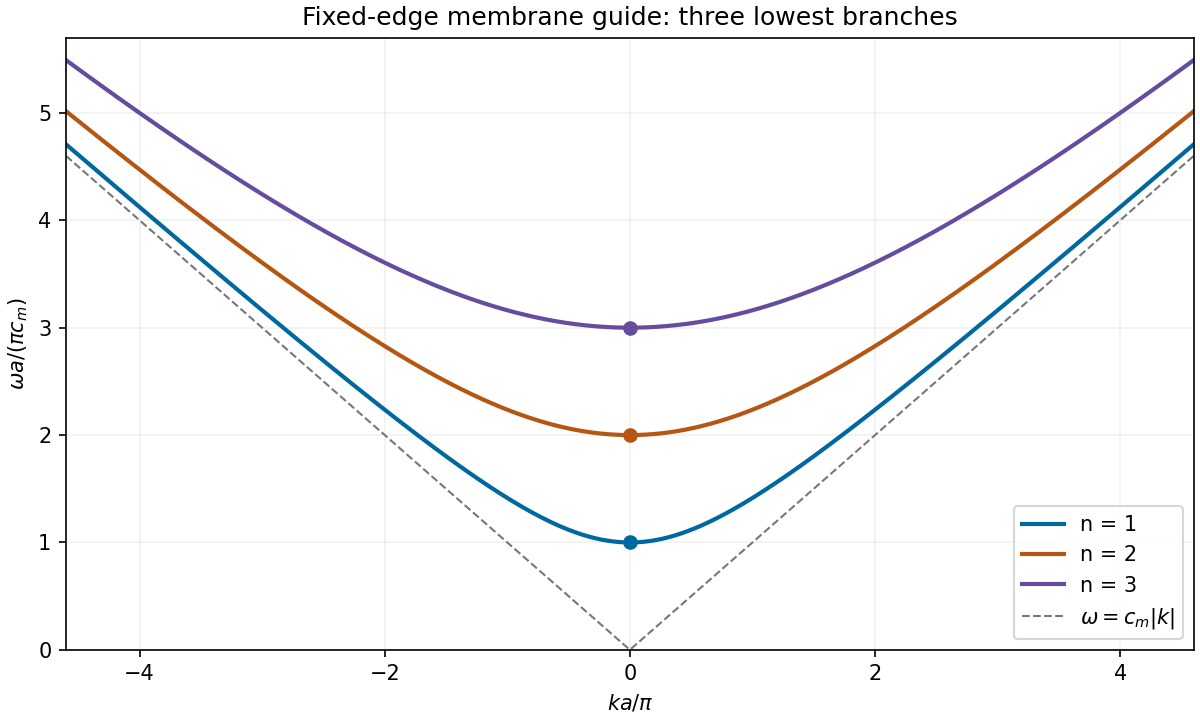
Three lowest membrane-waveguide dispersion branches, with their cutoffs and common large-wavenumber asymptote
. Details. For the th transverse mode, substitute into the membrane waveguide dispersion relation:Longitudinal propagation requires real nonzero , henceBelow the cutoff frequency of a membrane waveguide, , with , and a bounded excitation decays as rather than carrying a travelling wave along an infinite guide. At equality , the displacement has no longitudinal phase advance and the group velocity is zero; it is a cutoff oscillation, not a propagating mode carrying finite longitudinal power.
The fixed edge at is automatically satisfied by . At , the displacement must vanish at every , so . Thus the allowed transverse normal modes haveThe case gives zero displacement for this sine solution and is not a physical propagating mode. Negative only reverses the amplitude sign and does not create a distinct transverse mode. This discrete transverse spectrum is a consequence of the Dirichlet boundary conditions, rather than quantization of the longitudinal wavenumber in an indefinitely long guide.
For the trial displacement , direct differentiation givesThe two-dimensional wave equation is therefore satisfied ifHere is the longitudinal wavenumber, the transverse wavenumber, and the speed of an unconstrained membrane wave. The physical displacement is the real part, multiplied by an arbitrary displacement amplitude. has units and is surface mass density in , so has units as required.
A waveguide confines the transverse structure of a wave while permitting propagation along a chosen route. It can deliver energy to a distant receiver without the same geometric spreading as an unguided beam, protect a signal from unwanted coupling, and select transverse normal modes. It also makes propagation paths and coupling to devices more controllable. Confinement does not eliminate wave absorption or scattering loss, and it can introduce wave dispersion and cutoff frequencies of a membrane waveguide or corresponding cutoffs for other wave types.
Two examples are an optical fiber, which guides light by its core-and-cladding refractive index structure, and a hollow electromagnetic waveguide used to carry microwaves between a source and an antenna. A duct for acoustic waves is a further example. Each uses different material and boundary conditions, but the common idea is controlled transverse confinement.
Model the two openings as identical axis-aligned rectangles of width in , height in , and centre separation along . Their Fraunhofer diffraction field has the formThe original image shows first broad envelope zeros near and . The horizontal interference period is about ; the first interference minima near distinguish that fine scale from the envelope. The rectangular-aperture dimensions from diffraction zeros are thereforeThe edge-to-edge gap is . The long direction is vertical. These dimensions also explain the suppressed alternate principal array maxima: .
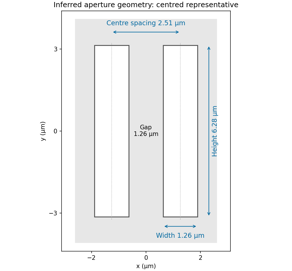
Inferred pair of rectangular openings, quantitatively labelled using the original angular-spatial-wavenumber axes
. Details. The factors are required by the stated convention; treating the plotted coordinates as cycles per micrometre would give different dimensions. The finite printed figure supports approximate dimensions. An overall translation and inversion of the aperture pair leave its Fourier intensity unchanged, so their absolute placement is not recoverable; the diagram chooses a convenient centred representative.
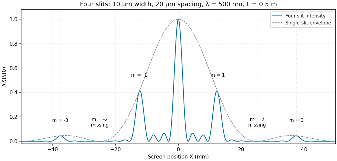
Let be horizontal position on the screen, , and use . The plotted interval is . With , and , the four-slit Fraunhofer diffraction intensity is the previous normalized expression evaluated at this angle. The total aperture width is , giving a Fresnel number of order , consistent with the far-field approximation.
Nominal principal array directions satisfy . Their screen positions areThus the visible nonzero orders are near , in addition to the central maximum. The even nonzero orders are missing diffraction orders: at the first envelope zero occurs at . The next envelope zero and direction lie at about , just beyond the screen edges.
At the nominal first and third array directions, and , respectively. The closest central minima satisfy , hence . Two small subsidiary array maxima occur between adjacent principal directions. The single-slit envelope slightly shifts the true off-axis maxima relative to the nominal principal array angles.


There are unlisted articles, also show them or only show them.