
Past exam of the quantum condensed matter course of the University of Cambridge 2014 3 Solution Created 2026-10-18 Updated 2026-10-20
Diagonalization and conventions. The spin-dependent part is . For a Hermitian Hamiltonian is real; the supplied lower-band spinor uses the convention , which will be adopted below. The squared spin matrix is . Hence the two ordered energies areIn the plane, let and . ThenIf , use to retain the energy ordering, and interchange the spin directions assigned below. This is an isotropic Rashba effect; has units of inverse length, whereas has units of energy times length.
Band minima. Define and . Completing the square givesAlong , the radial coordinate is , so the lower branch has two minima:In the full plane these are points on a circle of minima . Both branches meet at , . Their ordered energy curves contain : the lower curve descends from the crossing on either side, while the upper rises. Treating them as globally labeled smooth spin branches without switching labels across would obscure the lower-band minima.
Occupied regions and Fermi contours. At zero temperature each spin-split eigenstate with energy below is occupied. PutFor , . The lower-band roots are and , while the upper band is entirely empty. Thus the central disk is unoccupied, the annulus is singly occupied, and the exterior is unoccupied. Both Fermi circles belong to the lower band; there is no doubly occupied region.
At , the lower band is occupied for , giving a singly occupied disk with outer Fermi circle at . The two bands also meet the Fermi energy at the origin. That isolated degenerate point is not a finite doubly occupied disk, and occupation exactly at the Fermi energy is a boundary convention of zero area. Outside the outer circle the states are empty.
For , . The lower branch has outer radius , while the upper branch has inner radius . The disk is doubly occupied, with one state in each band at every momentum. The annulus is singly occupied, in the lower band only, and the exterior is unoccupied. These are the Fermi contours of an isotropic Rashba band; double occupancy here refers to two orthogonal spinor states at the same momentum, not two electrons occupying one identical quantum state.
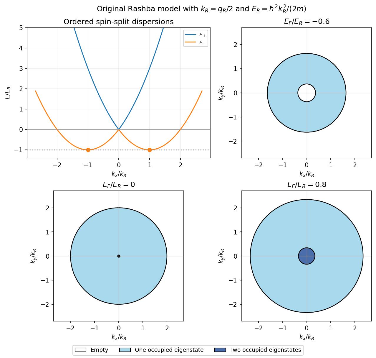
Rashba dispersion and occupied momentum regions below, at and above the band crossing
. Details. Inferring the splitting. Above the crossing, the two positive radii differ by :The minimum radius is therefore . It is the difference of the measured radii that is required for ; below the crossing the two lower-band radii instead add to .
Spinors and spin direction. Write , which has for . An orthogonal normalized partner to the supplied lower-band state isIndeed . Direct multiplication by the spin matrix gives eigenvalues and for and , respectively, so orthogonality has selected the other band rather than merely another arbitrary spin basis.
For a normalized spinor , the Pauli expectation values are . Consequently the Rashba spin texture isThe spin lies in the plane and is perpendicular to momentum. On the outer circle , which belongs to , it points clockwise as viewed from ; at it points along . On the inner circle , belonging to , it points counterclockwise; at it points along . Opposite momenta have opposite spins, consistent with time-reversal symmetry. At the origin the eigenstates are degenerate and no unique spin orientation is defined.
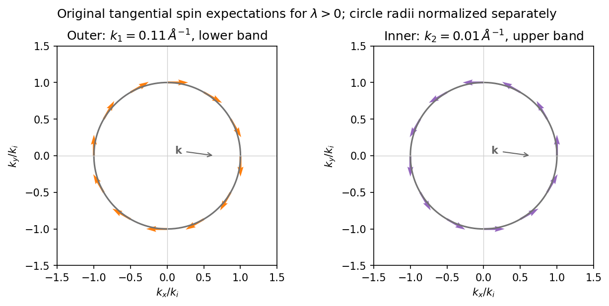
Opposite tangential spin textures on the outer lower-band and inner upper-band Fermi circles
. Details. Past exam of the quantum condensed matter course of the University of Cambridge 2013 4 Solution Created 2026-10-18 Updated 2026-10-20
Why degenerate perturbation theory is needed. If several unperturbed states have equal or nearly equal energy, a perturbation can mix them at leading order. In that subspace, diagonalize the perturbation matrix rather than using nondegenerate formulas with small energy denominators. The resulting eigenvectors identify the combinations selected by the coupling, and the eigenvalues give the leading splitting. Other remote states can then be included perturbatively.
For the linear combination of atomic orbitals description of molecular hydrogen, equivalent atomic states on the two nuclei supply the nearly degenerate starting functions. In an orthonormal two-state model, equal diagonal energy and real hopping give and symmetric/antisymmetric combinations. For actual overlapping atomic functions with overlap and Hamiltonian coupling , one instead solves a generalized eigenvalue problem:The bonding state has enhanced density between the nuclei and the antibonding state a separating node. Two opposite-spin electrons occupying the bonding molecular orbital describe the simplest closed-shell hydrogen-molecule bond. Electron-electron interaction and nuclear repulsion are needed to calculate a realistic total binding energy; the two-state splitting alone is not the full molecular energy.
In the nearly-free electron model, the analogous degenerate states are plane waves and at a Bragg scattering. A Fourier coefficient of the periodic potential couples them. At exact degeneracy , diagonalizing their two-by-two matrix givesThe associated standing waves place electronic density differently relative to the ionic potential. These are the same gap-opening combinations illustrated in Q1(b). The labels of the two starting basis states survive as mixed orbital or plane-wave character, rather than independent crossing eigenstates.
Origin of broad and narrow bands. Spatially extended s/p-derived orbitals have substantial overlap and therefore large hopping amplitudes and broad bands. More localized d orbitals overlap less strongly and produce narrower bands. A multiorbital tight-binding calculation assigns the on-site orbital energies and hopping matrices, forms Bloch sums, and diagonalizes the resulting matrix at each wavevector. Different hopping ranges and orbital symmetry determine the bandwidths and allowed interband coupling. The two-band description retains one broad combination and one nearly flat d-derived combination; a real transition metal contains several d orbitals and more complicated dispersions.
Hybridized eigenvalues and eigenstates. Let , in an orthonormal basis. Hermitian operator fixes the reverse coupling to be . Projection onto the two components givesSolving this quadratic yields the band hybridization dispersionFor nonzero , one eigenvector representation is , followed by normalization. Thus the wavefunctions exchange broad-band and d-band character through the avoided crossing; the levels are equal mixtures at the uncoupled crossing.
At , the parabola crosses the horizontal level at , with . For small nonzero , the curves avoid crossing with minimum direct separation . The lower branch follows the parabola below the crossing and flattens toward above it; the upper does the opposite. The lower branch satisfies everywhere and tends to from below as , while the upper branch always lies above . This is the perfectly flat-band continuum approximation, with zone-boundary intersections excluded as requested.
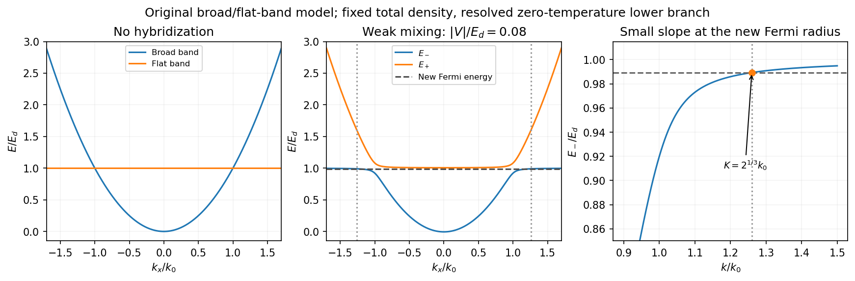
Uncoupled and weakly hybridized broad/flat bands, with the shifted Fermi radius and small lower-band slope
. Details. Fixed particle number and the larger Fermi sphere. Denote the uncoupled broad-band Fermi radius by to distinguish it from the new one . With two spin states, the broad-band number density at is . The stipulated equal population in the flat sector makes the total density twice that value. At zero temperature and any nonzero hybridization, all occupied states fit into the monotonic lower branch below , while the upper branch is empty. ThereforeThis is the stated factor increase. It uses fixed total particle number, equal spin counting, an exactly flat unhybridized band and enough available states below any Brillouin-zone restriction. In generic pairs of dispersive bands both hybridized pockets can remain occupied; then Fermi-volume conservation in two hybridized electron bands fixes a sum of volumes rather than this one radius. The exactly flat band is degenerate at , so its initial occupation must be specified, as it is here.
Fermi-velocity suppression. Set . The exact derivative of the lower branch isAt , and . For , the square bracket divided by two is . Since group velocity is and the broad-band reference velocity is ,so the flat-band hybridization Fermi-velocity suppression isThe reference velocity is that of the original broad-band Fermi sphere, not the broad-band slope at the larger ; omitting the radius change loses the factor .
The low-temperature qualification becomes more stringent as : the new chemical potential approaches with , and the relevant thermal energy must be small compared with this hybridization scale. At fixed nonzero temperature the singular flat-band redistribution is not automatically resolved for arbitrarily small coupling. A small but finite narrow-band dispersion can also change the occupation topology.
Density of states and magnetism. For an isotropic three-dimensional branch with spin degeneracy two,A small Fermi velocity therefore produces a large density of states. The localized, partially filled d-derived bands in iron, cobalt and nickel place many states close to the Fermi level; broad s/p-derived conduction bands in copper, silver and gold coexist with filled d bands lying below it. This explains the substantially larger Fermi-level density of states of the former group within the band picture. An exact factor of ten requires the actual band parameters and is not fixed by the two-band toy model.
A high density of states lowers the kinetic-energy cost of spin polarization. A repulsive exchange interaction can then satisfy the Stoner criterion and stabilize ferromagnetism. With a single-spin density of states and an on-site interaction normalization, the criterion is ; with spin-summed , it is . The large d-state contribution favors this instability in Fe, Co and Ni. The noble metals do not satisfy the corresponding instability condition in the same ordinary state; this does not imply that they have no weak magnetic response whatsoever.
Past exam of the quantum condensed matter course of the University of Cambridge 2013 3 Solution Created 2026-10-18 Updated 2026-10-20
Dopant atoms and carrier type. Substitutional semiconductor doping places a small fraction of foreign atoms on host lattice sites. In a tetrahedrally bonded group-IV semiconductor, a group-V substitution such as phosphorus in silicon has an extra valence electron. A shallow donor level just below the conduction edge can release that electron, leaving a positively charged donor. In an n-type semiconductor, mobile electrons are the majority carriers and the chemical potential shifts toward the conduction band.
A group-III substitution such as boron in silicon has one fewer valence electron. An acceptor level just above the valence edge captures an electron from the valence states, leaving a mobile electron hole and a negatively charged acceptor. In a p-type semiconductor, electron holes are the majority carriers and the chemical potential shifts toward the valence band. The material can remain electrically neutral in both cases: mobile carrier electric charge is compensated by fixed ionized impurity electric charge. Dopant freeze-out, compensation and degeneracy qualify the simplest one-carrier-per-dopant picture.
Making the junction. Choose p material at and n material at . Electrons initially diffuse from n to p, and electron holes from p to n, recombining near the interface. Negative ionized acceptors are exposed on the p side and positive ionized donors on the n side. They produce an electric field directed from n to p. The field opposes further majority-carrier diffusion until drift and diffusion balance and the equilibrium electrochemical potential is uniform.
The depletion regions are depleted of mobile majority carriers, not of the fixed dopant charges that create the space charge. At equilibrium the conduction and valence edges bend together, while the chemical potential is flat. The specified is a electric potential difference: the corresponding initial chemical-potential energy separation is . This convention is required by the quoted units and width formulas. Write for the absolute permittivity; the paper's is relative permittivity.
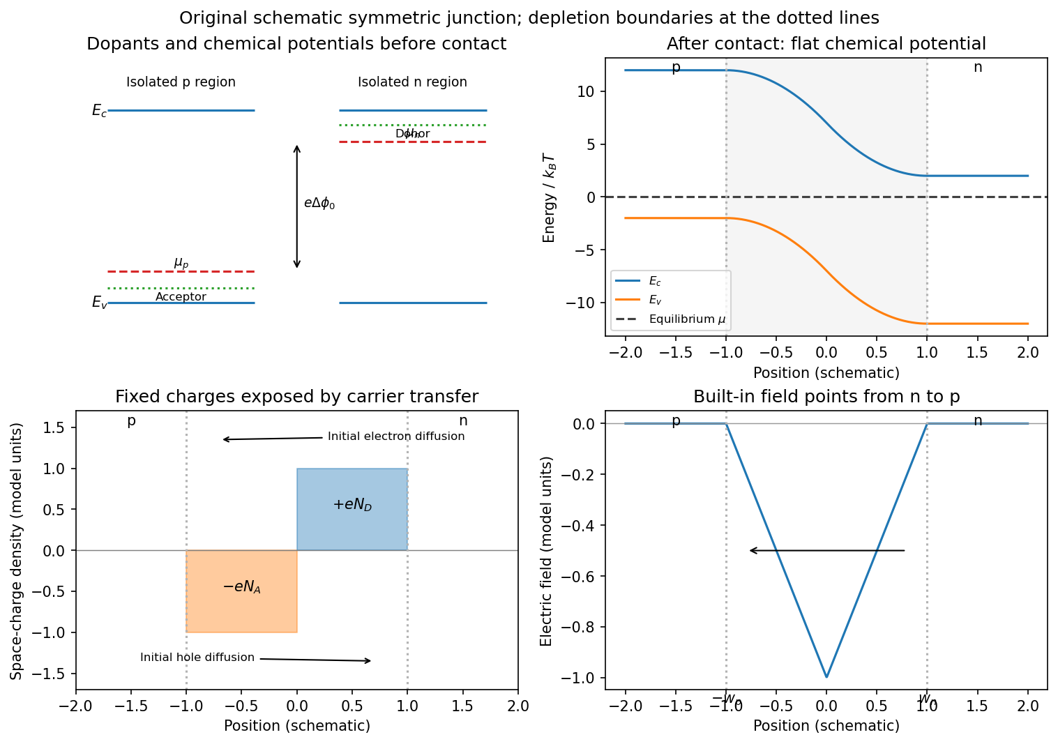
Substitutional donor/acceptor levels, equilibrium band bending, fixed space charge and the junction electric field
. Details. Poisson equation and widths. Let the depleted intervals be and . Fully ionized number densities correspond to electric charge densities , respectively. ThusThe factor converts a dopant concentration to a space-charge density. Requiring zero field in both neutral regions gives charge neutrality,With , direct integration gives the triangular fieldContinuity at the interface is the same neutrality condition. The field is negative throughout the depleted interval. Set . Its integral givesPotential continuity therefore requiresCombining it with neutrality yields the abrupt-junction depletion width and capacitance resultsThe more lightly doped side depletes farther, because equal and opposite space charges must be exposed.
Applied bias. Define positive as forward bias, raising the p-side terminal potential relative to the n-side terminal. It lowers the remaining barrier from to . Reverse bias has and raises that barrier. The same Poisson integration applies, with this replacement:Forward bias narrows the depleted region; reverse bias widens it. Under bias there need not be one equilibrium chemical potential across the device, so the equilibrium flat-level argument must not be reapplied unchanged. The barrier/width change is illustrated in the next figure.
Differential capacitance and electric charge sign. Put and . The signed p-side fixed electric charge per unit area isDifferentiating with respect to forward electric potential difference gives the positive capacitance per unit areaThe n-side electric charge is , so instead. If denotes a positive space-charge magnitude, the positive capacitance is for this forward-voltage convention. This resolves the sign implicit in the paper's positive . The total device capacitance is , where is its cross-sectional area.
Finite device and numerical sketch. For the symmetric device, and each side has thickness . Before full depletion,Using , the zero-bias width on each side is , less than . The total zero-bias capacitance is .
Full depletion occurs when , soAt larger reverse bias the depleted thickness cannot exceed . In the ideal fully depleted slab, incremental terminal electric charge changes the field uniformly through that fixed thickness, giving the full-depletion capacitance of a symmetric junction slabThus the idealized piecewise sketch over the specified range isIt is continuous at full depletion, rises through at zero bias, and has a formal inverse-square-root divergence as from below.
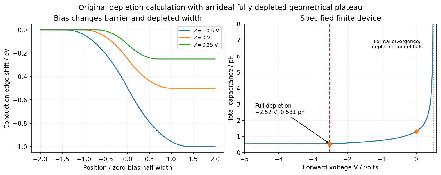
There are two physical limits to this extension. Once all dopants are exposed, their fixed space charge no longer increases, but the terminal electrodes can still acquire incremental electric charge; differentiating only the fixed ionized electric charge would incorrectly predict zero capacitance. Near , the depletion approximation itself fails as mobile carriers and forward injection become important, so the formal infinite endpoint is not a prediction of an actual infinite measured capacitance. The fully depleted plateau assumes ideal contacts and no breakdown, injection storage or extra series capacitance.
Past exam of the quantum condensed matter course of the University of Cambridge 2012 4 Solution Created 2026-10-18 Updated 2026-10-20
In the Lorentz oscillator model, each participating bound electron is displaced by an applied electric field against a restoring force. The model replaces complicated interband transitions by a driven damped harmonic oscillator. If is the electron displacement along the field and the electron charge is , its equation of motion isHere describes binding and describes loss of coherent motion. For , the complex amplitude isThe induced electric dipole moment is , so the electric polarization amplitude for number density isUsing givesThe paper's is this dimensionless relative permittivity, rather than the absolute permittivity . Independent classes of bound electrons contribute additive susceptibilities, usually with different resonance frequencies and optical oscillator strengths.
Writing separates the response intoAt zero frequency the real part is and the imaginary part vanishes. Near resonance the imaginary part has a positive photon absorption peak and the real part changes rapidly, passing through at . Above resonance the real part can become negative when damping is sufficiently weak; at very high frequency it approaches from below while the imaginary part tends to zero. Finite damping removes the undamped divergence.
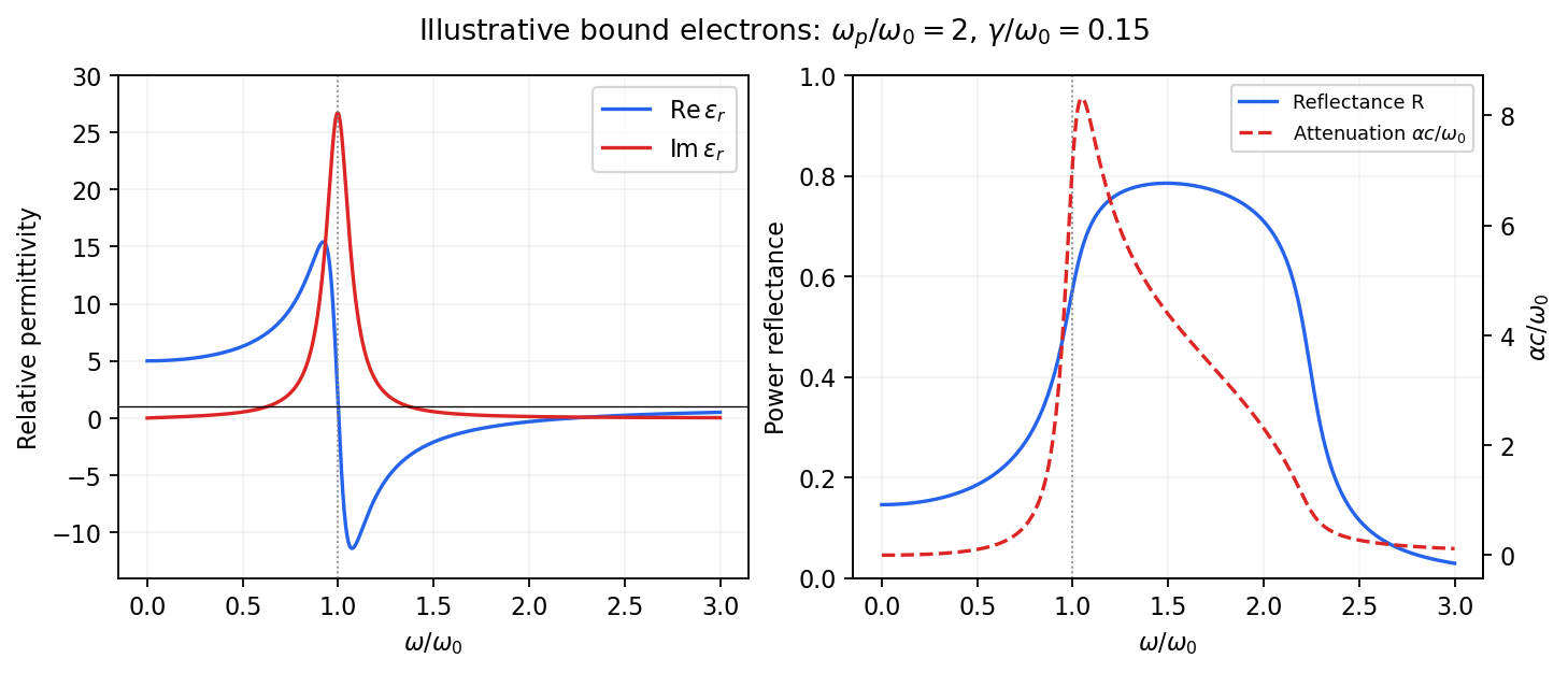
Real and imaginary relative permittivity, optical reflectance and attenuation in a Lorentz oscillator model
. Details. For a nonmagnetic material take the passive square-root branch , with . A plane wave then has an intensity attenuation coefficient . Thus the imaginary permittivity expresses dissipation, whereas the actual photon absorption coefficient is determined by the imaginary refractive index. The normal-incidence power reflectance isA large refractive-index mismatch produces wave reflection even without loss. In the undamped model between and , so the field is evanescent and wave reflection is total in a semi-infinite sample. With damping the response includes both wave reflection and photon absorption; a peak in the imaginary permittivity should not simply be identified with a reflectance peak.
To infer the short-wavelength background from , assume weak photon absorption and take the physical semiconductor branch . ThensoThis is an estimate of the valence-electron background in a frequency window above the doped-carrier response and below the effective bound-electron resonance. One reflectance value alone does not determine both parts of a complex dielectric constant. Even for real , a reciprocal-index branch gives the same ; the ordinary background index greater than unity selects the branch used here.
Using the supplied conventional cubic lattice parameter, the participating valence-electron number density isUsing for the stipulated free-electron comparison givesAn angular frequency “in eV” means its quantum energy , not . No doped-carrier effective mass should be inserted into this valence-electron count.
The low-frequency limit of the bound-electron contribution obeysConsequentlyThis effective resonance is much larger than the quoted band gap. There is no contradiction: the single oscillator has been assigned the strength of all sixteen participating valence electrons per conventional cell, whereas the band gap is only the lowest interband excitation threshold. A real spectrum distributes optical oscillator strength over many transitions. Equating the oscillator resonance to the lowest threshold would misrepresent the assumed background response. Here “low frequency” means low relative to ; the static response of the doped conducting sample also contains its free carriers.
The additional mobile carriers in doped indium antimonide contribute a Drude frequency response, obtained by setting their restoring frequency to zero. At infrared frequencies well below the effective valence resonance, the sum is approximatelyAt the shorter wavelengths the carrier term is small and approaches the background value. As wavelength increases, the negative free-carrier contribution lowers the real permittivity towards unity. For weak damping, refractive-index matching to vacuum gives the Drude-Lorentz reflectivity minimum atThis minimum is near , not its zero. At the slightly lower screened plasma frequency , the real permittivity crosses zero; at longer wavelengths it becomes negative and the material becomes strongly reflective. Finite damping prevents a perfectly vanishing minimum and rounds the edge. At still lower frequency the large conducting response also drives towards unity.
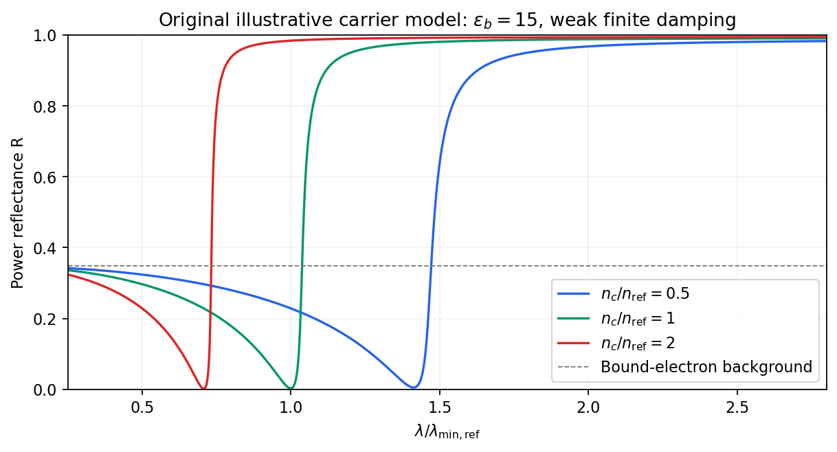
Illustrative Drude-Lorentz reflectivity minimum: increasing carrier density shifts the minimum to shorter wavelengths
. Details. For fixed carrier effective mass and background permittivity, and . The observed shift of the minimum towards shorter wavelength as doping increases is therefore the expected free-carrier trend. The figure is an original model illustration, not a digitization or quantitative fit of the supplied curves; the carrier effective mass, damping and their density dependence have not been specified.
Past exam of the quantum condensed matter course of the University of Cambridge 2012 3 Solution Created 2026-10-18 Updated 2026-10-20
Use two plane waves, and , as a basis near their Bragg degeneracy. The potential has Fourier coefficients ; its zero Fourier coefficient vanishes. All other plane waves are off resonance and are neglected in the leading nearly-free electron model. With , the Schrödinger equation reduces to the Hermitian matrix problemSetting the characteristic polynomial equal to zero givesSolving this quadratic equation givesFor the real cosine potential its coefficient is real; the absolute-value form also allows an arbitrary choice of origin and corresponding Fourier phase.
At the Brillouin-zone boundary, , the free energies are equal. The two standing waves have different probability densities relative to the lattice potential and are split byRepeating this avoided crossing at the reciprocal lattice boundaries joins smooth branches into energy bands. In one dimension a nonzero Fourier coefficient opens a gap at the corresponding crossing. In higher dimensions a direct gap at one wavevector need not give a common forbidden energy interval at every wavevector: different bands may still overlap in energy. The present two-dimensional example remains metallic even though the crossings are locally gapped.
For the rectangular lattice, choose real-space primitive vectors and . The reciprocal lattice vectors areDefine the half-widths of the first Brillouin zone by and . Their values and the zone areA primitive reciprocal cell can be drawn with a corner at the origin; its centred translate is the first Brillouin zone here. Its area is .
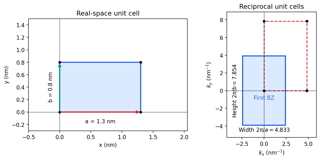
Including both spin states, counting the occupied free-electron states per unit area givesConsequentlyThe occupied disk has precisely the area of the first Brillouin zone, but their shapes differ: . It protrudes through both vertical zone boundaries and does not reach the horizontal ones. Thus two electrons per cell do not imply a filled first band in the absence of a separating band gap.
Fold the protruding caps by . The original circle and the translated circle intersect at , . The potential mixes these states and replaces each crossing by an avoided crossing. The lower branch reconnects into two open sheets running across successive zones in the direction; the upper branch forms a closed lens-shaped pocket about a vertical zone boundary. In a reduced-zone sketch its two halves sit at opposite edges, but periodic identification makes them one closed sheet. This is rectangular-lattice Fermi-surface reconstruction.
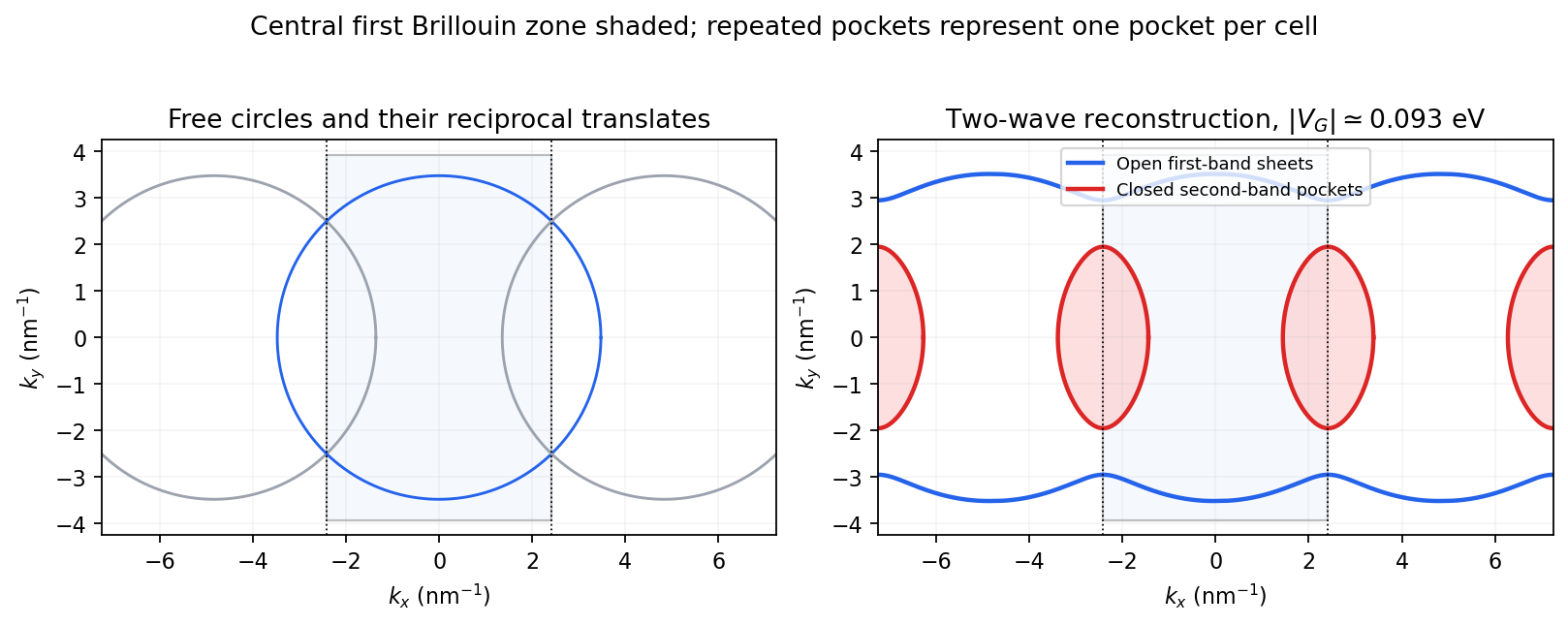


The largest pocket in this weak-potential construction is the lens-shaped intersection of two disks enclosed by the intersecting free circles. Each has radius and their centres are separated by . If , two sectors minus their two triangles give the lens bound on a reconstructed Fermi pocket:Opening a gap raises the upper branch at fixed chemical potential and shrinks its pocket. The reported quantum oscillation area satisfiesIt is therefore consistent with this closed sheet. Onsager quantization gives . An orbit on this closed contour can return to itself under the Lorentz force and occupy quantized Landau levels. The open sheets do not enclose a finite orbit area for a perpendicular field in this two-dimensional model. The observation is consistent with the reconstructed pocket, without uniquely determining a completely arbitrary band structure.
For a quantitative rough coupling estimate, use the supplied fixed-chemical-potential approximation and retain the two waves coupled by . WriteTheir upper eigenvalue isSetting it equal to gives the pocket boundaryIts intersection with occurs at , whereThe two-wave estimate of a Bragg-gap coupling from a pocket area therefore usesAt this reproduces the lens bound on a reconstructed Fermi pocket; the pocket disappears at . Numerical integration gives and . Matching the measured area gives , so the justified rough result isThis estimate neglects remote plane-wave admixtures and other Fourier coefficients. It also holds the chemical potential fixed as requested; an exact fixed-density calculation would determine it self-consistently after reconstruction. The numerical root is a way to implement the approximate model, not a measurement of to four significant figures.
There are unlisted articles, also show them or only show them.