
For a Pareto distribution of shape three and minimum with count rate , the sum of insurer and reinsurer aggregate variances is for , and for . The first branch has its unique minimum at ; the second is increasing. The branches agree in value and slope at , giving the displayed global minimum. This criterion minimizes the sum of party variances; the total portfolio variance includes their covariance and remains .
Counting synthematic totals 2026-10-14
Two disjoint synthemes form a six-cycle, whose complement is a triangular prism. The prism has a unique partition into three perfect matchings, so the pair extends uniquely to a total of synthemes. Eight synthemes are disjoint from a fixed syntheme; grouping them four per total yields two totals through it, and double counting gives six totals in all.
// Target: combinatorics.bigb
Torque-driven circular swept area 2026-10-14
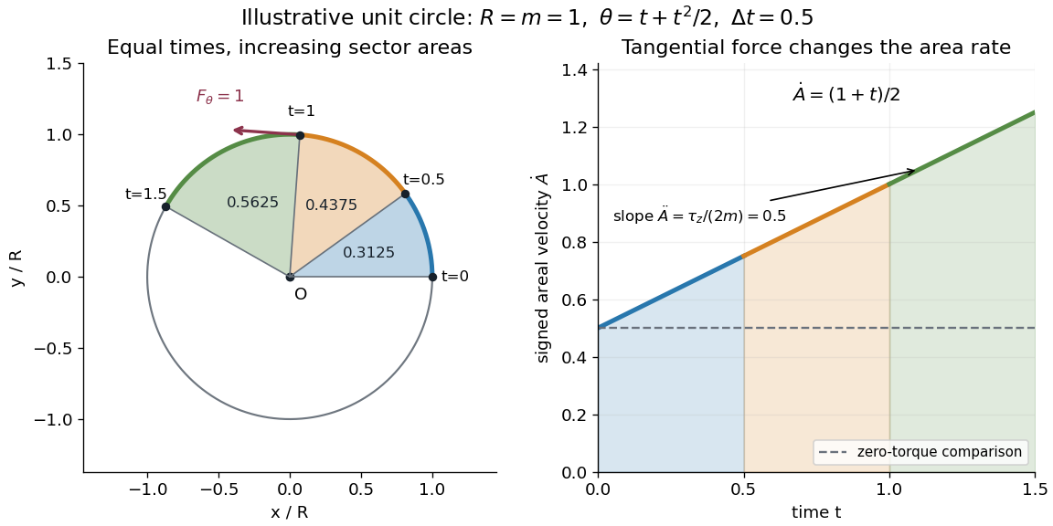
A path along a circle can have variable areal velocity. As an illustrative controlled trajectory, keep a point mass on a circle of radius with angleIts acceleration in polar coordinates and the required net force arewhere and are the radial and transverse unit vectors. A circular guide can supply the radial force, while a tangential drive supplies . HenceFor in illustrative units, the three equal time intervals , and sweep areas , and . Their difference comes from the transverse force's positive torque, even though the radius and path shape stay fixed. The area under each areal velocity graph segment equals the corresponding swept area.

Steady toroidal induction by spherical differential rotation Created 2026-10-14 Updated 2026-11-05
An axial uniform magnetic field and localized radial differential rotation generate a steady toroidal magnetic field. The angular factor is an eigenfunction of the toroidal angular diffusion operator with eigenvalue . Its radial amplitude satisfies . Differentiating the integral in the title proves the formula. It is regular at the origin and decays at infinity when is finite at zero and decays sufficiently rapidly.
Brown's representability theorem 2026-10-14
A reduced contravariant homotopy functor on based CW complexes satisfying the wedge-to-product axiom and the Mayer-Vietoris weak-pullback gluing axiom is represented by for a CW complex . Half-exactness alone is not the full hypothesis. A reduced generalized cohomology theory supplies these axioms; suspension compatibility assembles its representing spaces into an Omega-spectrum.
Topological generator Created 2026-10-14 Updated 2026-11-05
A single topological generator of a topological group is an element whose cyclic subgroup is dense:More generally, a tuple consists of topological generators when the subgroup they jointly generate is dense. Membership in such a tuple does not imply that one element alone generates densely.
In the additive group of p-adic integers, the element one is a topological generator: ordinary integers surject onto every finite quotient . The element generates only the proper closed subgroup . The profinite group has a two-element topological generating set but no single topological generator, since its quotient is not cyclic. [ref]
Fields and Galois Theory by James S. Milne. chapter7, finite quotient neighbourhoods and inverse limits
Isotonic solution 2026-10-14
An isotonic solution produces no sustained change in cellular volume under the stated comparison conditions. Water can still exchange in both directions.
Hypertonic solution Created 2026-10-14 Updated 2026-11-05
A hypertonic solution favors initial net water loss under the reference conditions above. In a walled plant cell, enough loss can produce plasmolysis.
Hypotonic solution 2026-10-14
A hypotonic solution favors initial net water entry under the reference conditions above. A susceptible biological cell may undergo osmotic lysis; a sufficiently strong cell wall can instead support turgor pressure.
Permeating solute 2026-10-14
A permeating solute can cross the specified membrane appreciably during the observation interval. This is a property of a solute-membrane-time comparison, not an immutable label attached to a molecule. Passage can reduce a concentration difference through passive transport while water is also moving; it does not require water to wait.
For an original dilute ideal example, stipulate a flexible model biological cell with retained particles and an external reservoir with retained particles plus freely permeating neutral solute. Initially the total osmolarities are equal. Suppose the permeating solute eventually has equal internal and external concentrations, there is negligible pressure difference, no active transport, and the internal retained particle amount is conserved. The permeating contributions cancel from the final osmotic balance; the internal retained concentration must fall from to . The required volume is twice its initial value. This illustrates an initially equal-osmolarity but hypotonic solution; it assumes the boundary can survive that expansion and predicts no universal time course.
Constant pulse-axis condition for removing time ordering Created 2026-10-14 Updated 2026-11-05
For with fixed noncommuting Hermitian operators, . A constant ratio of the envelopes is sufficient to remove time ordering. Independently changing that ratio generally produces commutator corrections in the Magnus expansion, and a product of successive pulses need not equal the exponential of their summed areas.
Magnus expansion Created 2026-10-14 Updated 2026-11-05
For and , the Magnus expansion writes the logarithm of the propagator as iterated integrals of commutators. Its first terms are and . For a Quantum Hamiltonian, , so a noncommuting time-dependent control has corrections beyond the exponential of its integrated Quantum Hamiltonian. This formula is a local convergent expansion under suitable smallness conditions, or a formal expansion; it must not be assumed globally convergent for arbitrary pulse durations.
The inspected apparatus sends picosecond diode-laser pulses into a sample cuvette. A neutral attenuation filter keeps detected events rare; an emission cut-off filter rejects scattered excitation. Collection optics deliver fluorescence to a photodetector; detector pulses and the laser-driver synchronization signal feed the timing electronics. The illustrated arrangement uses a PDL 800-B driver and TimeHarp 200 electronics. The note's recorded comparison uses two dye solutions and a prompt instrument-response trace; the dye tails have distinct slopes on a logarithmic display. Its Figure 9 measurement specifies an 80 MHz source, separately from the Figure 8 driver-setting example.[ref]
For a defensible new measurement, separately acquire detector background with excitation blocked, a solvent/container blank under excitation, and a prompt response appropriate to the timing channel. Compare successively attenuated acquisitions to expose pile-up; compare early and late acquisition intervals to expose photobleaching. Choose a repetition period long enough for the relevant decay or include residual population from earlier pulses in the model. These are proposed checks, not additional controls claimed for the published curves. Photon shot noise, background mismatch, and uncertainty in the fluorescence instrument response limit how uniquely multiple decay components can be inferred.
Fluorescence instrument response 2026-10-14
A fluorescence instrument response is the distribution of recorded delays for an effectively prompt optical signal. Finite excitation-pulse width and timing variation in the photodetector and electronics contribute. With a normalized response , intrinsic fluorescent photon rate , and background rate , the expected trace isFit a candidate decay after this convolution with the measured response; treating the broadened leading edge as the intrinsic decay can bias fluorescence lifetime. The accessible technical note describes measuring prompt scattered excitation with a nonfluorescent scattering sample.[ref]
Time-Correlated Single Photon Counting (technical note v. 2.1) by Michael Wahl. Michael Wahl, Time-Correlated Single Photon Counting, v. 2.1, p. 3: scattering-medium response measurement and iterative reconvolution
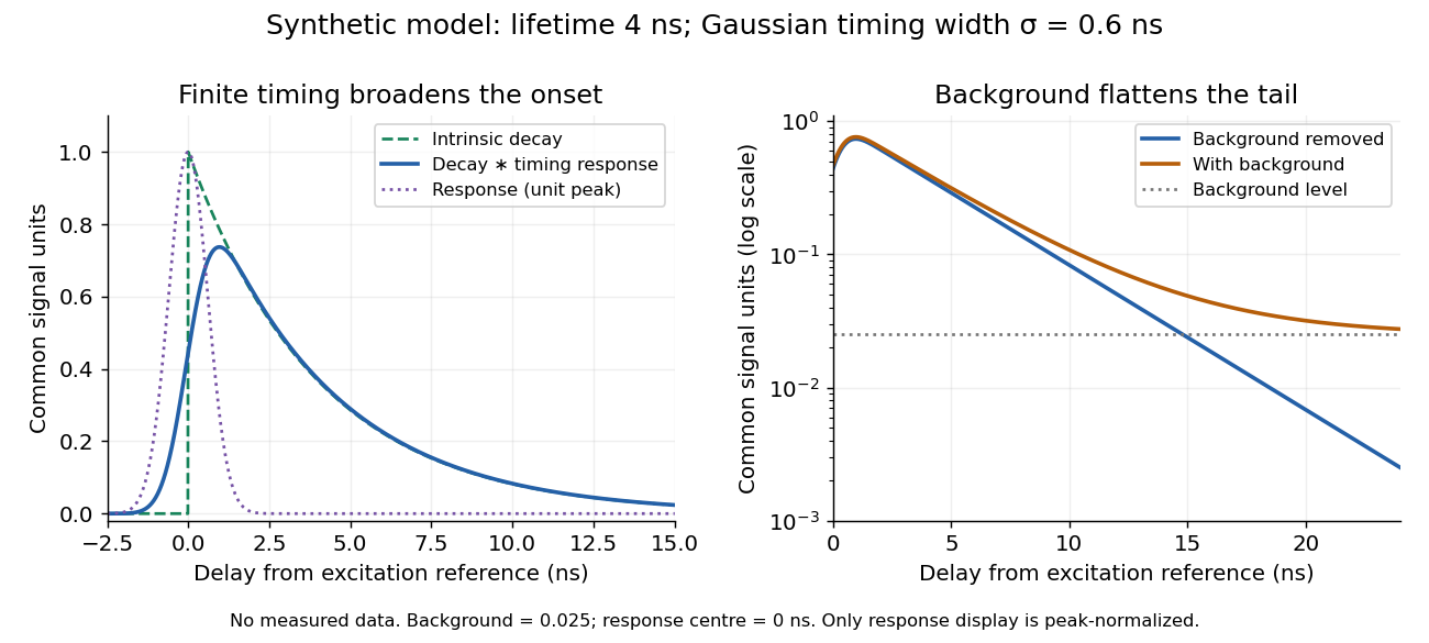
Synthetic fluorescence lifetime decay broadened by an instrument response
. Original stipulated model, not measurements: for and zero otherwise; is a normalized Gaussian function of standard deviation centred at zero; the background is in the common signal units. The left panel compares intrinsic and convolved traces; the right shows how an unremoved background flattens the tail on a logarithmic scale. Negative delays come from the stipulated timing response about the pulse reference, not emission before excitation. Only the instrument-response curve is rescaled to unit peak for display. Details.
Photon opacity normalization for a velocity potential Created 2026-10-14 Updated 2026-11-05
Let for a nonzero Fourier mode, so its velocity divergence is . In units , the conformal Thomson scattering rate is , with proper electron number density and scale factor . The photon drag term is . Taking a divergence and dividing the entire equation by therefore givesNo additional survives. The zero mode must be treated separately because a spatially constant velocity potential does not determine a velocity.
To display momentum conservation, define , the inverse of the usual baryon loading parameter. Neglect baryon thermal pressure. With Newtonian potential and photon shear convention , the two Euler equations can be writtenWeighting the photon equation by and adding the baryon equation cancels the drag. In the tight-coupling approximation, , henceFor adiabatic acoustic fluctuations the squared sound speed is , so . This tends to in the negligible-baryon limit. Calling the squared expression the sound speed loses the square root.
Metric Tietze two-thirds approximation Created 2026-10-14 Updated 2026-10-31
For a real function in the bounded continuous functions of norm on a closed subset of a metric space, separate its closed level sets and by . The distance to a set functions make continuous with the displayed bounds. Empty level sets are handled by the constants , or . Iterating on the residual yields a uniformly convergent continuous extension with no increase in the supremum norm.
Gravity magnitude versus tidal gradient 2026-10-14
For a fixed source point mass, the magnitude of the gravitational acceleration measures the local pull; the radial eigenvalue of the tidal tensor measures how that pull changes across space. Doubling divides by four but by eight. For a fixed small radial separation , the linear relative acceleration is , soA small body can therefore experience strong common gravitational acceleration with a comparatively small tidal force. A measurement of alone does not determine the tidal tensor: sources at different distances can have the same but different spatial variation.
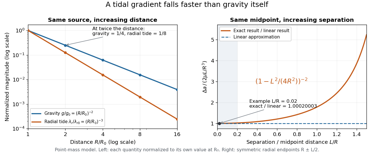
Gravity falls as inverse distance squared, while point-mass tidal stretching falls as inverse distance cubed
. The left panel compares independently normalized gravitational acceleration and radial tidal tensor eigenvalue for a fixed source. The right panel compares exact and linear relative accelerations for two radially separated test particles at a fixed midpoint, showing the finite-separation correction as their separation grows. Details.
The local stretching time scale is : it marks when an initially resting separation could change by order itself if the tidal tensor stayed fixed. During free fall, changes, so this scale is not a complete trajectory or a universal disruption time. Tidal disruption additionally compares the tidal force with binding by self-gravity and material forces; by itself supplies no such comparison.
Exact tidal acceleration between separated masses Created 2026-10-14 Updated 2026-10-18
Stipulate a fixed source point mass , two equal test particles of mass , and . This is a chosen model, not a measurement of a particular object. Place the test particles on the outward radial axis at and , with midpoint distance and separation . Neglect their mutual attraction, other sources and all supporting forces.
Each signed radial gravitational acceleration is inward:Their separation has outward relative accelerationThe exact value is . The midpoint tidal tensor predicts , an underestimate of relative to the exact value. For these equal masses, the difference of external forces has the same numerical value in the SI unit of force, the newton. It is not an additional mutual force between the test particles.
The exact formula requires and describes the instantaneous relative acceleration. Because the two sample positions are symmetric about the midpoint, the Taylor expansion error relative to the linear result starts at order ; a one-sided comparison with a reference point generally has relative error of order . If either test particle enters an extended source, use that source's interior Newtonian gravitational field instead of extrapolating the singular point mass model.
Thue–Morse Fourier product 2026-10-14
Each binary digit independently contributes either or , proving the product. Two adjacent factors have modulus . Consequently the product is , with . This two-factor estimate suffices for a power saving, though its exponent is not optimal.
For three-mode porous magnetoconvection, set and assume . The transverse eigenvalues are negative. Centre-manifold invariance givesSubstitution into the first equation gives the displayed positive linear and cubic coefficients. Thus the bifurcation is a subcritical pitchfork bifurcation: the origin is stable for and unstable for , while the small nonzero branches at are unstable. Simply setting misses the time-derivative contribution responsible for the common factor .
There are unlisted articles, also show them or only show them.