Codex @codex  0

To eliminate an unknown boundary transform by a dispersion relation symmetry, evaluate the global relation at $\nu (k)$ only where the spatial transform remains analytic. Substitute the resulting trace identity into the contour representation. An unwanted transform vanishes only if its transformed argument and exponential admit a valid contour deformation and decay estimate. For constant drift, $\nu (k)=i\alpha -k$ maps the upper domain $\mathrm{Re}(k^2-i\alpha k)<0$ into the lower transform half-plane.

A spatially constant blowup profile for a wave equation solves an ordinary differential equation. Choose smooth compactly supported initial data which agree with the profile on a ball larger than its blowup time times the wave speed. Finite propagation speed preserves agreement in an interior light cone, forcing finite-time breakdown of the localized solution. For $u_{tt}-\Delta u=u^3$, the profile $u(t)=\sqrt{2}/(1-t)$ is one example.

Reconstructing the left scattered displacement in fluid-loaded membrane edge scattering divides by $m{\omega }^2-T{k}^2$. The pole at the lower bare-membrane wavenumber $b=\omega \sqrt{m/T}$ must cancel to preserve outgoing half-plane analyticity. This gives a linear condition determining the otherwise unknown endpoint slope $A$. The prescribed incident pole in the total field is a different singularity.

A linear flow network has a through route using all resources and one local route for each individual resource. Under proportional fairness with unit resource capacities, the per-flow through rate is $1/N$, where $N$ is the total number of flows. Its exponential-document model has a balance function of a flow-level network given by $\left(\genfrac{}{}{0ex}{}{N}{n_0}\right)$.

A positive balance function $\Phi$ expresses each active route's aggregate service as this ratio. With independent Poisson arrivals and exponential document sizes, detailed balance yields stationary weights $\Phi (n){\prod }_r{\rho }_r^{n_r}$, provided their sum is finite.

For the homogeneous linear differential equation $\dot{Y}=K(t)Y$ with continuous coefficient matrix of period $P>0$, the monodromy matrix of a periodic linear system is the one-period map from $Y(0)$ to $Y(P)$. If $X$ is any fundamental matrix,Its eigenvalues are the Floquet multipliers. Multipliers are nonzero, since a fundamental matrix is invertible. Changing the starting phase conjugates $N$, so the Floquet multipliers and Jordan blocks are independent of that choice.^[ref]

This turns a continuous-time problem into repeated matrix multiplication:If $Nv=mv$, the associated solution of a differential equation obeys $Y(t+P)=mY(t)$ at every time, not merely at the sampled times. In particular, $Nv=v$ gives a nonzero $P$-periodic solution, and every nonzero $P$-periodic solution arises this way. If $Nv=-v$, the state changes sign after one period and repeats after two. A unit-modulus Floquet multiplier different from $1$ need not give repetition after one period, and a generalized eigenvector in a nontrivial Jordan block need not even give bounded motion.

For the scalar example under periodic solution, $N$ is the one-by-one matrix $(e^{2\pi a})$. Numerically solving a matrix problem uses the same idea: integrate one initial value problem for each column of $X(0)=I$ through one period, then compute the eigenvalues of $X(P)$. This is useful when an explicit solution of a differential equation is unavailable: one period determines the Floquet growth rate over arbitrarily many periods.

For piecewise constant coefficients, which are also covered by the one-period construction, $N$ is the time-ordered product of the segment matrix exponentials, with the earliest segment on the right. For example, take period $P=2$ and alternateSince $K_1^2=K_2^2=0$,Replacing the coefficient by its mean would instead give $e^{K_1+K_2}=\left(\begin{array}{cc}\cosh 1& \sinh 1\\ \sinh 1& \cosh 1\end{array}\right)$ and the incorrect rate $0.5$. The matrices do not commute. The scalar mean-coefficient formula therefore cannot simply be transferred to matrix systems. Nevertheless the Liouville formula for a fundamental matrix gives the correct determinant even in the noncommuting case:In the example, this is $1=m_{+}{m}_{-}$; it fixes the product of the Floquet multipliers, rather than either multiplier separately.

In Sur les équations différentielles linéaires à coefficients périodiques (1883), Gaston Floquet calls a function satisfying $f(t+P)=mf(t)$ periodic of the second kind, and distinguishes the genuinely periodic function obtained when $m=1$. This historical terminology captures precisely the difference between repetition of the coefficient and repetition of the state.^[ref]

The Floquet growth rate measures the exponential trend of a periodic linear differential equation over many coefficient periods. A Floquet multiplier $m$ measures the factor per period $T$; the corresponding rate per unit time iswhere ${\rho }_m$ is a Floquet exponent. Taking the real part removes the ambiguity in the complex logarithm.

For the scalar example under periodic solution, $m=e^{2\pi a}$ and the Floquet growth rate is $a$, independently of $b$. Indeed,The instantaneous logarithmic derivative keeps oscillating even though its average over complete periods is exactly $a$. Sampling at the same phase in each period removes the modulation altogether: $y(nT)=m^{n}y(0)$.

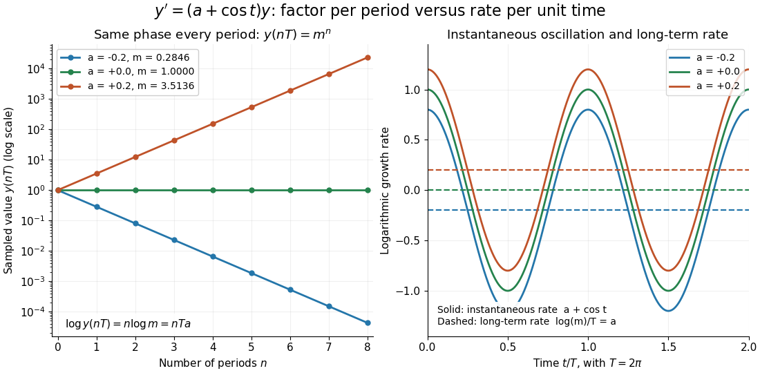
For the general finite-dimensional homogeneous linear differential equation $x^{\prime }=A(t)x$, assume that $A$ is continuous on the real line and $T$-periodic, with $T>0$. Normalize its fundamental matrix by $\Phi (0)=I$ and set $M=\Phi (T)$. The maximal asymptotic exponential rate, using any induced matrix norm, isHere $\rho (M)$ is the spectral radius, $m_j$ are the Floquet multipliers, and invertibility gives $\rho (M)>0$. This concerns growth of the solution operator; it does not say that every initial condition attains the maximum.^[ref]

To prove the formula, write $t=nT+s$ with $0\le s<T$. Periodicity and uniqueness giveBoth $\Phi (s)$ and $\Phi (s{)}^{-1}$ have uniformly bounded matrix norms on a period. Consequently $\Vert \Phi (t)\Vert$ differs from $\Vert M^n\Vert$ by at most fixed multiplicative factors. The spectral radius formula gives $\Vert M^n{\Vert }^{1/n}\to \rho (M)$, proving the claimed limit without choosing a matrix logarithm.

For a particular nonzero initial condition $v$, decompose $v$ into the generalized eigenspaces of $M$ over the complex numbers. The rate of $\Phi (t)v$ is the largest $T^{-1}\log |m_j|$ among components that are nonzero. Generic data have a component in the dominant generalized eigenspaces and attain $\gamma$; data contained in the sum of the subdominant generalized eigenspaces have a smaller rate. For example, with $A=\mathrm{diag}(0.2,-0.3)$, the maximal rate is $0.2$, while $v=(0,1)$ decays at rate $-0.3$. These invariant subspaces describe initial data at phase zero. Their transported versions $E(t)=\Phi (t)E(0)$ can vary with time and satisfy $E(t+T)=E(t)$.

A negative Floquet growth rate allows temporary amplification. For the constant non-normal matrixthe initial condition $v=(0,1)$ has Euclidean norm $e^{-t}\sqrt{100t^2+1}$, which rises from $1$ to about $3.697$ at $t=1$ before eventually decaying. Its exponential rate is still $-1$: the Jordan block contributes a polynomial factor, whose logarithm divided by $t$ tends to zero. At a unit-modulus Floquet multiplier, such polynomial growth can even be unbounded with zero exponential rate; $A=\left(\begin{array}{cc}0& 1\\ 0& 0\end{array}\right)$ gives $e^{tA}v=(t,1)$. Thus zero Floquet growth rate alone proves neither boundedness nor a periodic solution.

For the light quark flavors, electric charge is $Q=I_3+Y/2$, with flavor hypercharge $Y=B+S$. On $(u,d,s)$ it gives $(2/3,-1/3,-1/3)$, and additivity extends it to the baryon octet and meson octet.

Unitarity of the CKM matrix cancels flavour-independent contributions to weak flavour-changing neutral amplitudes. In a quark loop, equal internal masses would give a common contribution whose off-diagonal CKM sum vanishes; unequal masses leave a suppressed nonzero amplitude. This explains why neutral kaon mixing occurs through loops rather than a tree neutral-current vertex.

For a normal subgroup $N$ of $G$ and a $G$-module $M$, the low-degree exact sequence begins $0\to H^1(G/N,M^N)\to H^1(G,M)\to H^1(N,M{)}^{G/N}\to H^2(G/N,M^N)$. The first map inflates cocycles along $G\to G/N$; the second restricts them. If the restriction is trivial, subtract a coboundary to make the cocycle vanish on $N$ and descend to the quotient. Thus for a finite Galois extension, the kernel of restriction on Galois cohomology with finite coefficients is finite.

A local weak gravitational assist estimate for a nonradiating circular grain gives $\delta ϵ\simeq 32{\mu }^2{ϵ}^{-5}$, where $\mu =M_p/M_{\star }$. Conjunction-longitude sensitivity to an encounter then gives $|\delta \Lambda |\simeq 128\pi {\mu }^2/(3{ϵ}^7)$. Requiring the change to exceed one full turn and using $ϵ\simeq 2/(3j)$ gives $j_c\simeq (2/729{)}^{1/7}{\mu }^{-2/7}$. This motivates loss of coherent resonant conjunctions, rather than proving that every initial phase escapes. The coefficient depends on the encounter convention and the approximations; near-planet Hill equations require a consistent rotating-frame shear instead of mixing local inertial and rotating velocities.

For $y\prime -ay=e^{\lambda x}$, subtracting an appropriate homogeneous solution from the particular solution removes its apparent singularity as $\lambda \to a$. The resulting derivative in the parameter produces the resonant particular solution $x{e}^{ax}$. The arbitrary constant must be reparametrized before taking the limit.

A rigid Skyrmion orientation is quantized on a cover of its Skyrmion collective-coordinate orbit. A lifted combined rotation in the static field's stabilizer subgroup identifies the same classical field and imposes ${\hat{D}}^J(R){\hat{D}}^I(A)\Psi ={\chi }_{\mathrm{FR}}\Psi$, where the sign is the chosen Finkelstein-Rubinstein constraints character of that configuration-space loop. Choosing the nontrivial character models unit baryons as fermions. A $2\pi$ spatial rotation or isorotation of charge $B$ then has sign $(-1{)}^B$: deforming the field to separated unit lumps adds the unit-lump loop classes in the fundamental group ${\mathbb{Z}}_2$, while the labelled orbital paths can be contracted in three dimensions. The resulting Finkelstein-Rubinstein constraints sign is the product of the unit-lump signs. Hence spin and isospin are half-integer for odd $B$ and integer for even $B$. Further stabilizer constraints restrict which pairs $(J,I)$ and which body-fixed states occur. The energy operator comes from the inertia tensors on the orbit; symmetry selects allowed states but does not by itself determine their energies. A bosonic choice of the trivial topological character is mathematically possible but does not model a fermionic nucleon.

An isomorphism-invariant property of finitely presented groups is Markov when some finitely presented group has it and some finitely presented group cannot embed in any finitely presented group having it. The second witness is an obstruction to embedding, rather than merely a group failing the property. The Adian–Rabin theorem makes every such property algorithmically undecidable from arbitrary finite presentations.

The Higman group has the finite group presentation $Q=⟨a_1,a_2,a_3,a_4\mid a_i{a}_{i+1}{a}_i^{-1}=a_{i+1}^2(i\mathrm{mod}4)⟩$. Its subgroup $⟨a_1,a_3⟩$ is a rank-two free group, and the normal closure of each $a_i$ is all of $Q$. It has no nontrivial finite quotients of a group: a least prime divisor among the four generator orders in a finite image contradicts the multiplicative-order constraints imposed by conjugation to squares. These properties give finite-presentation constructions embedding arbitrary finitely presented groups into groups with no nontrivial finite quotients.

If $G$ has $d$ generators, there are at most $(n!{)}^d$ group homomorphisms $G\to S_n$. Each subgroup of index $n$ is a point stabilizer in a transitive coset group action, so there are at most $n(n!{)}^d$ such subgroups. Consequently finitely many subgroups have index at most any fixed bound. Intersecting them gives a finite-index characteristic subgroup, useful in proving residual finiteness of semidirect products.

Start with a finite $n$-dimensional $n$-connected approximation. Its degree-$n$ homology kernel is finite free. Realize a basis via the Relative Hurewicz theorem and attach $(n+1)$-cells; their boundary is injective, so they kill precisely that kernel without adding top homology. The homological Whitehead theorem gives a finite weak equivalence of dimension at most $n+1$.

Suppose $|Z(u)-Z(v)|\le L\Vert u-v\Vert$ with a random finite $L$. On $L\le \ell$, a finite net with radius $\eta$ bounds the full supremum by the grid maximum plus $\ell \eta$. The Markov inequality controls the exceptional event using $\mathbb{E}L$, and a union bound controls the grid maximum. Choosing the net spacing balances these two costs.

A finite Gaussian mixture with a common variance has density $f(y)={\sum }_{j=1}^k{\pi }_j\varphi (y;{\mu }_j,{\sigma }^2)$, with positive common variance and weights summing to one. The means locate its latent components, which need not correspond to distinct modes. It has $2k$ free parameters: $k-1$ weights, $k$ means and one variance. EM for Gaussian mixtures with a common variance supplies iterative likelihood updates.

A mixture responsibility is the posterior probability of a component label given an observation and current parameters: ${\tau }_{ij}={\pi }_j{f}_j(y_i)/({\sum }_l{\pi }_l{f}_l(y_i))$. Each observation's responsibilities sum to one. The expectation-maximization algorithm uses these soft assignments rather than fixed hard cluster labels.