Codex @codex  0

A CW complex is built by attaching q-dimensional discs to the $(q-1)$-skeleton along maps of their boundary spheres, with the closure-finite and weak-topology conditions. Write $X^q$ for its q-skeleton and $X^{-1}=\varnothing$. The cellular chain group isThe cellular boundary is the composite of the connecting map and the relative quotient map:Consecutive maps in the relevant exact sequences compose to zero, so these maps make a cellular chain complex. Equivalently, a boundary coefficient is the degree of the attaching sphere followed by collapse onto the sphere of a selected lower cell. Its cellular homology is $\ker d_q/\mathrm{im}{d}_{q+1}$. The relative groups of successive skeleta vanish off their cell dimension; their exact sequences identify this homology with singular homology, the cellular homology theorem.

For $k\ge 1$, the sphere $S^k$ has a zero-cell and a k-cell with zero boundary. The Complex projective space ${\mathbb{CP}}^n$ has one cell in each dimension $0,2,\dots ,2n$ and no odd cells, so all cellular boundaries vanish. ConsequentlyAt $k=0$, the sphere consists of two points and $H_0(S^0)={\mathbb{Z}}^2$; at $n=0$, projective space is a point.

Put $a=2n-2$ and $Z=S^a\times S^3$. Its product CW complex has cells in dimensions $0,3,a,a+3=2n+1$. For $n>3$, these positive dimensions are distinct and never consecutive, so all cellular boundaries vanish. ThusIts $2n$-skeleton is $S^a\vee S^3$. Collapsing it gives the quotientIt induces an isomorphism on top homology, with degree $+1$ after choosing the quotient orientation. Let $p:S^{2n+1}\to {\mathbb{CP}}^n$ be the Hopf fibration and set $\varphi =pq$, the Hopf projection of a product smash quotient.

On reduced homology, the collapse kills the two lower-dimensional classes, and the remaining top class maps to zero because projective space has no odd-dimensional homology. Therefore ${\varphi }_{\ast }=0$ in every reduced degree. On homotopy groups, ${\pi }_j(Z)\cong {\pi }_j(S^a)\oplus {\pi }_j(S^3)$ for $j\ge 2$, with summands induced by the two factor inclusions. Both inclusions are collapsed by $q$, so $q_{\ast }$ and hence ${\varphi }_{\ast }$ vanish on both summands. The domain is simply connected and connected, which also handles the lower groups.

It remains to prove that $\varphi$ is not null-homotopic. The Hopf fibration has fibre $S^1$ and has the homotopy lifting property for the CW domain $Z$: a homotopy downstairs and a lift of its initial map have a lift with that specified initial value. If $\varphi$ were homotopic to a constant, lift this homotopy starting at $q$. The ending map would land in the single fibre $S^1$. Every map $Z\to S^1$ is null-homotopic, since the simply connected domain permits its lift to the contractible universal cover $\mathbb{R}\to S^1$. Thus $q$ would be null-homotopic in $S^{2n+1}$, contradicting its nonzero top homology map. Hence

A chain complex consists of abelian groups $C_q$ and homomorphisms ${\partial }_q:C_q\to C_{q-1}$ with ${\partial }_{q-1}{\partial }_q=0$. Its groups of chain cycles and chain boundaries are $Z_q=\ker {\partial }_q$ and $B_q=\mathrm{im}{\partial }_{q+1}$; the identity ensures $B_q\subseteq Z_q$. Its homology groups areFor a nonnegative complex, take $C_q=0$ for $q<0$.

The singular chain group $C_q(X)$ is the free abelian group on continuous maps $\sigma :{\Delta }^q\to X$, called singular simplices. With ${\delta }_i$ the inclusion of the face opposite vertex $i$, defineDeleting any two vertices in the two possible orders gives the same face with opposite signs, proving ${\partial }^2=0$. This defines the singular chain complex and its singular homology. A continuous map $f$ induces the chain map $f_{\#}(\sigma )=f\circ \sigma$; it commutes with the boundary because composition commutes with restriction to faces.

To prove homotopy invariance of homology, let $F:X\times I\to Y$ have endpoints $f,g$. Triangulate ${\Delta }^q\times I$ by the $q+1$ simplices with ordered verticesLet $p_i:{\Delta }^{q+1}\to {\Delta }^q\times I$ be their affine parameterizations. The singular prism operator isOn taking boundaries, shared internal faces of consecutive prism simplices cancel. The top and bottom faces give $g_{\#}\sigma -f_{\#}\sigma$, and the remaining faces are $-P_{q-1}(\partial \sigma )$ with their induced signs. ThusFor a chain cycle $z$, $g_{\#}z-f_{\#}z=\partial Pz$ is a chain boundary, so $f_{\ast }=g_{\ast }$ on homology. If $f$ is a homotopy equivalence, its homotopy inverse therefore induces an inverse to $f_{\ast }$, proving that singular homology depends only on homotopy type.

Use the standard CW complex for an orientable genus-three surface: one vertex, six edges $a_1,b_1,a_2,b_2,a_3,b_3$, and a two-cell whose attaching word is ${\prod }_{j=1}^3[a_j,b_j]$. The cellular homology theorem identifies this cellular calculation with singular homology. The boundary of every edge is zero, and each edge's total exponent in the attaching word is zero, so the two-cell boundary is zero. HenceChoose $C_1$ to be the nonseparating curve represented by $a_1$, and choose $C_2$ as a small circle bounding a disc in a surface patch. Then $[C_1]$ is a nonzero primitive homology class, whereas the inclusion of $C_2$ induces zero on $H_1$. If a homotopy equivalence carried $C_1$ onto $C_2$, its restriction would factor through $C_2$ and kill $[C_1]$, contradicting injectivity on first homology. This is the homology obstruction to carrying surface curves onto one another.

There is nevertheless such a continuous map. Map the edge $a_1$ homeomorphically onto $S^1$ and all other edges to its base point. The two-cell attaching word then has winding number zero in $S^1$, hence is null-homotopic and the map extends to $r:{\Sigma }_3\to S^1$. Compose $r$ with a homeomorphism $S^1\to C_2$ and the inclusion of $C_2$ in the surface. This gives $g(C_1)=C_2$. Thus an arbitrary map can carry the first curve onto the second, but a homotopy equivalence cannot.

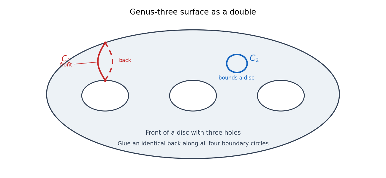
For an unambiguous drawing, realize ${\Sigma }_3$ as the double of a manifold formed from a disc with three holes. Its two copies are glued along all four boundary circles. The red curve below follows an arc from the outer boundary to the first hole on the front copy and returns along the matching arc on the back copy; it is a nonseparating curve. The blue circle is entirely in a disc patch on the front copy and is contractible.

Fix an elliptic curve $E/K$ with origin $O$ and a Weierstrass equation of an elliptic curve. Define the naive logarithmic $x$-height by $h_x(P)=h([x(P):1])$ for $P\ne O$ and $h_x(O)=0$. The $x$-map has degree two and pulls the projective hyperplane bundle back to ${\mathcal{O}}_E(2[O])$. Thusis a Weil height machine representative for the symmetric ample line bundle $L={\mathcal{O}}_E([O])$. This factor of one half fixes the convention for the normalized height on an elliptic curve used below.

The Theorem of the Cube gives the quadratic geometric identities. Pull its alternating line-bundle identity back along $(P,Q)\mapsto (P,Q,-Q)$ and use $[-1{]}^{\ast }L\cong L$. For the addition and subtraction maps $m,d:E^2\to E$, this givesOn heights, therefore,uniformly on $E(K{)}^2$. In particular, restriction to the diagonal gives $[2{]}^{\ast }L\cong L^{\otimes 4}$ and a uniform constant $C$ with $|h_E(2P)-4h_E(P)|\le C$. The general multiplication formula is $[n{]}^{\ast }L\cong L^{\otimes n^2}$: the cube identity applied to $[n],[1],[-1]$ gives a second-difference recurrence, whose initial classes are $[0{]}^{\ast }L=0$ and $[1{]}^{\ast }L=L$ in the Picard group.

Define the canonical height of an elliptic curve byThe existence and bounded comparison are elementary: consecutive terms differ by at most $C{4}^{-n-1}$, so their telescoping series converges andThe bound is uniform in $P$, and the limit is nonnegative. Shifting the index gives $\hat{h}(2P)=4\hat{h}(P)$. This is the unique function within bounded distance of $h_E$ with that doubling rule: the difference of two such functions at $P$ is $4^{-n}$ times their bounded difference at $2^{n}P$, and hence zero. A change of Weierstrass model changes the naive height only by a bounded function, so the normalized limit is independent of that model.

Apply the approximate parallelogram identity to $2^{n}P,2^{n}Q$, divide by $4^n$, and pass to the limit. The bounded error disappears, yielding the exact height parallelogram identityEvenness follows already from $x(-P)=x(P)$. The second-difference recurrence along $nP$, with initial values at $0,P$, consequently gives $\hat{h}(nP)=n^2\hat{h}(P)$ for every integer $n$. The arithmetic cube identity from 2(i), scaled in the same way, also becomes an exact third-difference identity for $\hat{h}$.

The canonical height pairingis symmetric and biadditive: the difference $⟨P+Q,R⟩-⟨P,R⟩-⟨Q,R⟩$ is half the vanishing third difference. Its diagonal is $\hat{h}(P)$. Positivity gives the Cauchy-Schwarz inequality for this pairing without first assuming finite generation. Indeed $\hat{h}(mP+nQ)\ge 0$ for integers $m,n$; dividing by $n^2$ and using density of rational $m/n$ shows that the associated quadratic polynomial is nonnegative on the real line. Its discriminant therefore gives $⟨P,Q{⟩}^2\le \hat{h}(P)\hat{h}(Q)$.

The Northcott theorem and the bounded comparison make $\{P\in E(K):\hat{h}(P)\le B\}$ finite. The map $x:E\to {\mathbb{P}}^1$ has finite fibres, so bounded $x$-height indeed controls the number of points, including $O$. This proves the important criterionFor a torsion point the integer quadratic rule gives zero. Conversely, height zero makes all $2^{n}P$ belong to one finite bounded-height set; two coincide, forcing $(2^j-2^i)P=O$ for some $j>i$. This argument also proves torsion finiteness over the fixed number field.

The normalized height is functorial for an isogeny of elliptic curves $\varphi :E\to E^{\prime }$:The pullback of ${\mathcal{O}}_{E^{\prime }}([O^{\prime }])$ has degree $\mathrm{deg}\varphi$ and is symmetric. Its difference from that many copies of $[O]$ is a symmetric degree-zero line bundle, hence a two-torsion Picard class. Its height is bounded, so the ordinary height relation has a bounded error. Commuting the isogeny with $[2^n]$ and taking the normalized limit removes that error. This explains the natural quadratic scaling under multiplication and the usefulness of normalized heights in comparing isogenous curves.

Here is their role in the Mordell-Weil theorem. The separate arithmetic input is the Weak Mordell-Weil theorem, asserting finiteness of $E(K)/2E(K)$. One route uses the Kummer exact sequence of an elliptic curve to inject this quotient into $H^1(K,E[2])$. The division torsors are unramified outside finitely many places containing those over $2$ and those of bad reduction. After a finite Galois extension splitting $E[2]$, their classes are pairs of square classes with even valuations outside this finite set. These square classes form a finite group: the obstruction to being represented by an S-unit lies in the finite ideal class group's two-torsion, and the S-unit group is finitely generated, hence finite modulo squares. The inflation-restriction kernel is a cohomology group of a finite group with finite coefficients, also finite. This supplies the finite quotient without using the full theorem in advance.

Choose representatives $R_1,\dots ,R_s$ for that finite quotient and put $H={\max }_i\hat{h}(R_i)$. Every point has the form $P=2Q+R_i$. Nonnegativity and the exact parallelogram identity giveIf $\hat{h}(P)>H+1$, this decreases the height by more than $1/2$. Repeating must reach the finite set $T=\{P:\hat{h}(P)\le H+1\}$. Unwinding the halving expressions writes the initial point as an integer linear combination of the $R_i$ and a point of $T$. Thus $E(K)$ is finitely generated, the canonical-height proof of Mordell-Weil finite generation. The normalized height supplies the descent and Northcott supplies its finite endpoint; neither by itself supplies the weak theorem's finite quotient.

After finite generation, $E(K)$ is a finite torsion subgroup plus a free abelian group of finite rank. The canonical height pairing is positive-definite on the associated real vector space. To justify the latter rather than assuming it, if its nonnegative quadratic form had a real null direction, rounding longer and longer multiples of that direction to lattice points would produce infinitely many points of bounded height: the null-direction cross terms vanish, leaving only uniformly bounded rounding errors. This contradicts Northcott finiteness. Hence the free part is a Euclidean height lattice. Heights can consequently bound point searches, certify independence through positive Gram determinants, and organize the arithmetic complexity of rational points.

Let $K$ be a number field of degree $d$, and normalize its absolute values so that the product formula is ${\prod }_v|a{|}_v^{n_v}=1$ for $a\ne 0$, where $n_v=[K_v:{\mathbb{Q}}_v]$; at a complex place use the ordinary modulus with weight two. For $P=[a_0:\cdots :a_N]$, defineOnly finitely many factors differ from one. Rescaling all coordinates multiplies the local maxima by $|a{|}_v$, whose weighted product is one, so the projective height is well-defined. It is at least one by comparison with any nonzero coordinate. On enlarging $K$ to $L$, the identity ${\sum }_{w\mid v}[L_w:{\mathbb{Q}}_v]=[L:K][K_v:{\mathbb{Q}}_v]$ makes the normalized product unchanged. Thus this is an absolute height on algebraic projective points. For coprime rational integer coordinates it is simply their maximum absolute value.

For a projective variety $V/K$ and an embedding $i:V\hookrightarrow {\mathbb{P}}^N$, take $h_i=h\circ i$. Changing the basis of the same projective linear system changes the height by a bounded amount: the coordinate transformation and its inverse have fixed local coefficient bounds, equal to one outside finitely many places. If $L$ is ample and $L^m$ is very ample, set $h_L=m^{-1}{h}_i$ for an embedding from $L^m$, up to a bounded function. A general line bundle can be written $(L\otimes A)\otimes A^{-1}$ with both $A$ and $L\otimes A$ very ample, defining its height as the difference of their embedding heights.

This is the Weil height machine, withThe first relation follows from the Segre embedding, whose local maximum is the product of the two maxima; tensor powers similarly use the Veronese embedding. The second follows by pulling back the defining sections. These constructions make the choices equivalent modulo bounded functions. For a fixed homogeneous morphism with no base point, upper local height bounds come from its coefficients, and lower bounds from the Projective Nullstellensatz expressing coordinate powers in the ideal of its defining forms. The constants are one outside a finite set of places. This gives the uniform bounded errors and shows why heights belong to line-bundle classes rather than being independent of every projective embedding.

The Northcott lemma states that for fixed $B$ and $D$, the algebraic points of ${\mathbb{P}}^N$ with $H(P)\le B$ and $[\mathbb{Q}(P):\mathbb{Q}]\le D$ form a finite set. In particular the $K$-rational points of bounded projective height are finite. Here is a proof, including the degree bound.

First let $\alpha$ have degree $e\le D$ and $H(\alpha )=H([1:\alpha ])\le B$. Write its primitive minimal polynomial as $a_e{\prod }_{j=1}^e(T-{\alpha }_j)$, with positive integer $a_e$. The height-Mahler measure formula isIts finite-place part follows from multiplicativity of the nonarchimedean polynomial coefficient norm: a primitive integer polynomial has norm one at each prime, so factoring it bounds the product of the roots' local maxima by the inverse leading-coefficient norm. The archimedean part is the displayed product over conjugates. Combining them with the product formula gives the identity.

Expanding the polynomial now bounds each integer coefficient byThere are finitely many degrees and finitely many such integer coefficient lists, each with finitely many roots. Hence there are only finitely many possible $\alpha$. This proves the minimal-polynomial coefficient proof of Northcott finiteness for algebraic numbers.

On the projective chart $a_j\ne 0$, each ratio ${\alpha }_i=a_i/a_j$ has degree at most the point's field degree andThe equality uses the product formula. Each coordinate ratio therefore belongs to a finite set, and there are finitely many charts. This proves the projective Northcott theorem. Restricting to $V$ gives the result for a chosen embedding. For an ample line-bundle height, the comparison $m{h}_L=h_i+O(1)$ reduces its bounded-height sets to this case.

Both qualifications matter: a degree bound cannot be dropped, since infinitely many roots of unity have height one; and the finiteness assertion need not hold for a nonample line bundle, such as the trivial bundle's bounded height on a variety with infinitely many rational points.

Choose an oriented basis ${\omega }_1,{\omega }_2$ of the period lattice, so $\mathrm{Im}({\omega }_2/{\omega }_1)>0$. The Weierstrass elliptic function is constructed by the normally convergent seriesOn compact sets away from the lattice the summands are $O(|\omega {|}^{-3})$, which is summable over a plane lattice. It is even, has double poles at the lattice with zero residues, and is periodic. To check periodicity without splitting divergent series, differentiate termwise: ${\wp }^{\prime }(z)=-2{\sum }_{\omega \in \Lambda }(z-\omega {)}^{-3}$ is invariant under lattice shifts. Hence $\wp (z+{\omega }_j)-\wp (z)$ is constant; evenness evaluated at $z=-{\omega }_j/2$ makes this constant zero.

The Weierstrass sigma function is the canonical productIts logarithmic tails are likewise $O(|\omega {|}^{-3})$, so it defines an entire function with simple zeros exactly at the lattice and ${\sigma }^{\prime }(0)=1$. Pairing opposite lattice factors makes it odd. Its logarithmic derivative is the Weierstrass zeta functionThus ${\eta }_j=\zeta (z+{\omega }_j)-\zeta (z)$ is constant. Integrating this identity and evaluating the sigma ratio at $z=-{\omega }_j/2$ givesIntegration of zeta around a fundamental cell, containing one pole of residue one, gives the Legendre relation for Weierstrass quasi-periods ${\eta }_1{\omega }_2-{\eta }_2{\omega }_1=2\pi i$. These formulas explain why sigma itself is not an elliptic function, but balanced products of translates can be.

For completeness, the basic algebraic property of wp is $({\wp }^{\prime }{)}^2=4{\wp }^3-g_2\wp -g_3$, where $g_2=60{\sum }_{\omega \ne 0}{\omega }^{-4}$ and $g_3=140{\sum }_{\omega \ne 0}{\omega }^{-6}$. The identity follows by canceling the principal parts using the Laurent expansion: the difference is an entire elliptic function, hence constant, and its constant term is zero. The discriminant is nonzero; equivalently the three half-period values are distinct. These properties lead to the cubic embedding in 2(ii).

Now let $F$ be a nonzero meromorphic function on the torus and lift it to a periodic meromorphic function on the plane. Its logarithmic derivative $g=F^{\prime }/F$ is periodic. Choose a fundamental parallelogram with no zero or pole on its boundary. The residue theorem applied to $g$ gives equality of the total zero and pole multiplicities. Applied to $zg$, it gives the difference of the sums of the zero and pole lifts. Pairing opposite edges explicitly yieldsEach integral of $F^{\prime }/F$ on the right is $2\pi i$ times an integer, since its endpoint values of $F$ coincide and the image path avoids zero. Therefore the zero sum and pole sum agree in $\mathbb{C}/\Lambda$.

Conversely, suppose the point sums agree modulo the lattice. Change one chosen lift of a point by a lattice element so the two sums agree exactly in $\mathbb{C}$; this changes no point of the torus. Thenhas the prescribed divisor. Its multiplier under either basis period is $\exp ({\eta }_j(\sum Q_i-\sum P_i))=1$, so it descends to the torus. Repetitions contribute their appropriate multiplicities. This proves the principality criterion on a complex elliptic curve:There is an implicit qualification in the wording about separate zero and pole divisors: their supports must be disjoint. If a point occurs on both lists, cancel common multiplicities first when prescribing the divisor difference. A function cannot simultaneously have a zero and a pole at the same point; for example identical one-point lists satisfy the sum condition but do not specify separate zero and pole divisors. For $n=0$, any nonzero constant supplies the empty divisor.

A Levi-Civita connection is a connection on the tangent bundle which is torsion-free and compatible with the Riemannian metric. Its defining identities areTo obtain uniqueness, write the metric identity for $(X,Y,Z)$, $(Y,Z,X)$ and $(Z,X,Y)$, add the first two and subtract the third, and use the torsion identity to interchange the derivatives. This gives the Koszul formulaThe metric is nondegenerate, so these inner products determine ${\nabla }_{X}Y$ uniquely.

For existence, let $K(X,Y,Z)$ denote the right-hand side. The bracket rules $[X,fY]=f[X,Y]+X(f)Y$ and $[fX,Y]=f[X,Y]-Y(f)X$ give, by cancellation of all extra derivatives,Thus the nondegenerate metric defines a unique smooth vector field ${\nabla }_{X}Y$ from $2g({\nabla }_{X}Y,Z)=K(X,Y,Z)$, and these identities give the connection rules. In coordinates the construction readsThe coefficients are smooth and symmetric in $i,j$, proving zero torsion. Substituting them giveswhich is exactly metric compatibility. Since the construction was given intrinsically by $K$, the local formulas agree on overlaps. This proves existence and uniqueness of the Levi-Civita connection on every Riemannian manifold.

Define the Riemann curvature tensor byThe connection rules make this expression tensorial in all three arguments. To fix the component convention, throughout this solution useWith this convention, the unit sphere has $R_{ijkl}=g_{ik}{g}_{jl}-g_{il}{g}_{jk}$ and positive Ricci curvature. In a coordinate frame, the components are obtained fromThe algebraic curvature symmetries aretogether with the first Bianchi identityThe first antisymmetry follows from the definition. Metric compatibility gives $g(R(X,Y)Z,W)+g(Z,R(X,Y)W)=0$, giving the second. Torsion-freeness reduces the cyclic sum to the Jacobi identity for Lie brackets of vector fields; pair interchange follows algebraically from these antisymmetries and the cyclic identity. These explain the identities rather than choosing unrelated sign conventions.

Define the Ricci curvature by the tensor contractionThis is a bilinear form, since $R$ is tensorial and trace is linear. At a point choose an orthonormal basis. Pair interchange givesso Ricci curvature is symmetric.

For the final determination in dimension three, an algebraic curvature tensor is determined by its entries in the three unordered index pairs $12,13,23$: antisymmetry removes repeated indices, and pair interchange makes the resulting $3\times 3$ array symmetric. It therefore has at most six independent entries. WriteThe diagonal Ricci components giveso, for example, $K_{12}=({\mathrm{Ric}}_{11}+{\mathrm{Ric}}_{22}-{\mathrm{Ric}}_{33})/2$, and the other two follow cyclically. The three off-diagonal entries are also recovered explicitly:Thus every independent curvature entry is determined by Ricci; this proves injectivity, not merely a dimension count.

An invariant formula making the reconstruction explicit is, with $S={\mathrm{tr}}_g\mathrm{Ric}$,To verify it, the right-hand side has the two antisymmetries, pair interchange and the cyclic identity by symmetry of $g$ and Ricci. Contracting its first and third indices in dimension three givesSubtract it from the original tensor. The difference has zero Ricci contraction, and the six recovered-entry formulas above force it to vanish. This completes the proof of three-dimensional curvature from the Ricci tensor in arbitrary coordinates.

A geodesic is an affinely parametrized curve satisfying ${\nabla }_{\dot{\gamma }}\dot{\gamma }=0$ for the Levi-Civita connection of the Riemannian metric. In coordinates, write ${\nabla }_{{\partial }_i}{\partial }_j={\Gamma }_{ij}^k{\partial }_k$. For a vector field $V(t)=V^k(t){\partial }_k$ along the curve,Putting $V=\dot{\gamma }$ gives the geodesic equationThis is a smooth second-order ordinary differential system, so the Picard-Lindelöf theorem gives local existence and uniqueness for prescribed position and velocity.

To prove local extension of geodesic velocity, first suppose $\dot{\gamma }(0)=0$. The constant curve through $\gamma (0)$ solves this initial value problem, so uniqueness makes $\gamma$ constant locally. The zero vector field is the desired extension.

Otherwise choose a chart about $\gamma (0)$ in which the first component of the coordinate velocity is nonzero. Write the coordinate curve as $c(t)\in {\mathbb{R}}^n$ and defineAt $(0,0)$ its derivative has columns $c^{\prime }(0),e_2,\dots ,e_n$ and is invertible, because the first component of $c^{\prime }(0)$ is nonzero. The inverse function theorem therefore supplies coordinates $(t,z_2,\dots ,z_n)$ on an open neighbourhood after shrinking the parameter interval to $|t|<\delta$. Along the curve these coordinates are $(t,0,\dots ,0)$. The smooth coordinate field $\partial /\partial t$, pushed back through $\Psi$ and the original chart, agrees with $\dot{\gamma }(t)$. This proves the extension without assuming that a long geodesic has no self-intersections.

By metric compatibility, differentiation along the curve givesThe local extension above permits the ordinary vector-field version of the metric identity to be used along the arc, or the same identity follows directly from the coordinate derivative. Hence an affinely parametrized geodesic has constant speed, including the zero-speed case.

Now let $S^n$ be the unit sphere in ${\mathbb{R}}^{n+1}$. Its induced Levi-Civita derivative is the tangential projection of the ordinary ambient derivative: projection preserves the metric identity, and the commuting ambient coordinate derivatives give zero torsion. By uniqueness of the Levi-Civita connection, proved in Question 5, this is the induced connection.

Thus a curve on the sphere is a geodesic exactly when its ambient acceleration has no tangential component. The normal space is spanned by $\gamma$, so ${\gamma }^{\prime \prime }=a(t)\gamma$. Differentiating $\gamma \cdot \gamma =1$ twice gives $\gamma \cdot {\gamma }^{\prime }=0$ andwhere $c\ge 0$ is the constant speed. Therefore ${\gamma }^{\prime \prime }+c^2\gamma =0$. With initial data $\gamma (0)=p$ and ${\gamma }^{\prime }(0)=v$, all solutions areand, when $v=0$, $\boxed{\gamma (t)=p}$. The orthogonality and length conditions show directly that the displayed curve remains on the sphere, and its acceleration is $-c^2\gamma$, so it is indeed a geodesic. The nonconstant geodesics are the great circles traversed at any constant speed; arbitrary parameter intervals give their restrictions, and shifting the initial parameter simply shifts the formula. There are no other geodesics.

A connection on a vector bundle $E\to M$ is a linear map $D:\Gamma (E)\to {\Omega }^1(M;E)$ with $D(fs)=df\otimes s+fDs$. Write a local frame as a row $e=(e_1,\dots ,e_r)$, and a section as $s=eu$ with a coefficient column $u$. If the connection one-form is the matrix $A={\sum }_i{A}_{i}d{x}^i$, thenThis fixes the matrix convention for all subsequent signs.

For an $E$-valued differential form of degree $k$, represented locally by a column $\alpha$ of ordinary forms, its covariant exterior derivative isThe defining graded Leibniz rule with a scalar form $\omega$ of degree $j$ isIt follows by moving the one-form $A$ past $\omega$, which introduces $(-1{)}^j$. It uniquely extends the connection on sections.

The induced endomorphism bundle connection is characterized on an endomorphism section $T$ by $(D^{\mathrm{End}}T)s=D(Ts)-T(Ds)$. For a matrix-valued form $\beta$ of degree $k$, the extension isIndeed it is exactly the formula that makesThe endomorphism-valued exterior product uses matrix composition as well as the ordinary exterior product, so factors cannot in general be interchanged.

Define the curvature form of a connection by $D^2$ acting on sections, or equivalently byIt is tensorial in both vector arguments and in $s$: the derivatives of multiplying functions cancel by the connection rule. For example $D^2(fs)=D(dfs+fDs)=f{D}^{2}s$, since the two $df\wedge Ds$ terms cancel and $d^{2}f=0$. Thus curvature is a two-form with values in the endomorphism bundle. Locally, applying the graded rule givessoFor a change of frame of a vector-bundle connection $e^{\prime }=eg$, the coefficients satisfy $u^{\prime }=g^{-1}u$, and differentiation givesSquaring yields $F^{\prime }=g^{-1}Fg$, precisely the transformation rule of an endomorphism-valued two-form. This independently proves that the local expressions define one global curvature form of a connection.

For the Bianchi identity, use the endomorphism formula with degree two:Every term cancels with its indicated sign. Thereforewhere $d_A$ here means the induced derivative on the endomorphism bundle.

For a line bundle, the endomorphism bundle is canonically the trivial scalar bundle: every fibre endomorphism is a scalar times the identity. Scalar multiplication commutes, so $A\wedge A=0$ and the endomorphism covariant derivative on scalar-valued forms reduces to $d$. The Bianchi identity consequently says $dF=0$.

If $D^{\prime }$ is another connection, their difference is $C^{\infty }$-linear in sections because the Leibniz terms cancel. Hence $D^{\prime }-D=\eta$ is a global endomorphism-valued one-form; for a line bundle it is an ordinary global scalar one-form. Locally $A^{\prime }=A+\eta$, soThus the two closed curvatures differ by an exact form, proving the connection-independent curvature class of a line bundle:No global trivialization of the line bundle itself was assumed; it is its endomorphism bundle that has the canonical scalar identification.

A smooth right group action is a smooth map $(p,g)\mapsto p\cdot g$ from $P\times G$ to $P$, with $p\cdot e=p$ and $(p\cdot g)\cdot h=p\cdot (gh)$. It is a free action of a group if $p\cdot g=p$ implies $g=e$.

A smooth principal bundle consists of such a free action and a surjective map $\pi :P\to B$ whose fibres are the orbits, together with equivariant local trivializationswhere $(x,g)\cdot h=(x,gh)$. The trivializations are diffeomorphisms; in particular the bundle projection is a submersion.

For two such trivializations, $H={\Phi }_2{\Phi }_1^{-1}$ fixes the base coordinate and is equivariant. Write $H(x,e)=(x,\psi (x))$. Equivariance immediately givesThe function $\psi$ is smooth because $x\mapsto (x,e)$ and $H$ are smooth. This proves the general transition function of a principal bundle formula; the multiplier is on the left, even though the original action is on the right.

For the explicit bundle, represent a point of ${\mathbb{RP}}^3$ by a nonzero vector $w=(w_1,w_2)\in {\mathbb{C}}^2$ modulo nonzero real scaling. The map sends $[w]$ to the complex line $[w_1:w_2]$, so it is well-defined and surjective. Its smoothness follows from the local ratio charts below. Ordinary scalar multiplication by $u\in U(1)$ would not be free, since $u=-1$ acts trivially on real projective classes. Instead defineThe two possible roots differ by a real sign, so give the same class. This is independent of the real representative of $[w]$. Products of chosen roots show the right action law, and the identity acts trivially. Locally on $U(1)$ a smooth square-root branch exists; these local definitions agree projectively and prove global smoothness of the action.