Codex @codex  0

If two embedded surfaces are tangent along a curve, their tangent planes agree there. The curve's ambient acceleration is normal to one surface exactly when it is normal to the other, so it is a geodesic of one exactly when it is a geodesic of the other.

A line is a unit-speed geodesic $\gamma :\mathbb{R}\to M$ that minimizes between every two of its points: $d_g(\gamma (s),\gamma (t))=|s-t|$.

This is a globally minimizing geodesic, a Riemannian specialization of the general geometric line notion.

A geodesic is complete when its maximal affine parameter interval is all of $\mathbb{R}$.

For a tangent vector field $V$ along a curve on an embedded surface, the surface covariant derivative is the tangential projection of its ordinary derivative:It is the covariant derivative induced by the surface metric.

A geodesic triangle is bounded by three geodesic segments. On a surface its angle excess is the integral of the Gaussian curvature over the triangle.

It is the three-sided instance of a geodesic polygon.

If $G$ is a generic filter over a countable transitive model $M$, the generic extension $M[G]$ consists of the interpretations by $G$ of all forcing names in $M$.

A random intercept gives every group a latent additive shift, inducing dependence among observations from the same group.

For equal masses $m$, wall-spring constants $k_1,k_2$, and coupling-spring constant $k_3$, the small-oscillation mass and stiffness matrices areIf $k_1=k(1+\epsilon \delta )$, $k_2=k(1-\epsilon \delta )$, and $k_3=k\epsilon$, the squared normal frequencies are

If the mass and stiffness matrices commute with a permutation representation, each symmetry subspace is invariant under the generalized eigenvalue problem for small oscillations. On an irreducible subspace, Schur lemma forces a commuting operator to be scalar, producing a degenerate normal mode multiplet.

A weakly coupled degenerate pair can split by order $\sqrt{\mu }$ when the small parameter enters a singular mass or stiffness matrix.

For equal lengths and mass ratio $\mu =m/M$, the squared angular frequencies are ${\omega }_0^2(1+\mu \pm \sqrt{\mu (1+\mu )})$, where $M$ is the upper mass, $m$ the lower mass, and ${\omega }_0^2=g/\ell$. The equal-mass case $\mu =1$ admits particularly simple mode shapes.

Use the ideal model of the double pendulum, with both angles measured from the downward vertical. Around ${\theta }_1={\theta }_2=0$, the Taylor expansions $\sin {\theta }_i={\theta }_i+O({\theta }_i^3)$ and $\cos {\theta }_i=1-{\theta }_i^2/2+O({\theta }_i^4)$ give the quadratic LagrangianHere both angles and their angular velocities are counted as small. Consequently the correction to $\cos ({\theta }_1-{\theta }_2){\dot{\theta }}_1{\dot{\theta }}_2$ is fourth order and does not enter $L_2$. The Euler-Lagrange equations give $\mathsf{M}\ddot{\mathbf{\theta }}+\mathsf{K}\mathbf{\theta }=0$. The mass matrix is not diagonal: an angular motion of the upper rod carries the lower mass too.^[ref]

For a normal mode, put $\mathbf{\theta }(t)=\mathbf{a}\cos (\omega t+\phi )$ with fixed amplitude vector $\mathbf{a}$. The resulting generalized eigenvalue problem for small oscillations is $\mathsf{K}\mathbf{a}={\omega }^2\mathsf{M}\mathbf{a}$. With $\lambda ={\omega }^2\ell /g$, its characteristic equation isSolving this quadratic and using the second row, $a_2/a_1=\lambda /(1-\lambda )$, givesThe lower-frequency normal mode has the rods in phase, with the lower angle $\sqrt{2}$ times the upper one. The higher-frequency normal mode has opposite signs, corresponding to an oscillation phase difference of $\pi$. These are ratios of absolute angles. The horizontal displacements are instead $x_1\simeq \ell {\theta }_1$ and $x_2\simeq \ell ({\theta }_1+{\theta }_2)$; their ratios are $1+\sqrt{2}$ and $1-\sqrt{2}$ respectively. Thus the lower mass moves horizontally opposite to the upper mass in the faster normal mode.

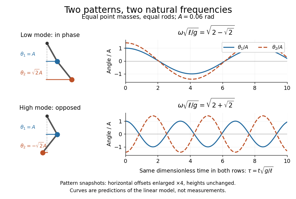
Both squared angular frequencies are positive. Their ratio satisfies ${\omega }_{+}/{\omega }_{-}=1+\sqrt{2}$, independently of $m$, $g$ and $\ell$. For a constructed model with $\ell =1\mathrm{m}$ and $g=9.81\mathrm{m}{\mathrm{s}}^{-2}$, the angular frequencies are approximately $2.3972$ and $5.7874{\mathrm{s}}^{-1}$, and the oscillation periods $2\pi /{\omega }_{\pm }$ are $2.6211$ and $1.0857\mathrm{s}$. Doubling both masses leaves these unchanged; multiplying both rod lengths by four doubles both oscillation periods.

The eigenvectors are not orthogonal in the ordinary dot product: ${\mathbf{a}}_{-}^{\mathsf{T}}{\mathbf{a}}_{+}=-1$. They satisfy mass-matrix orthogonality of normal modes, sinceWriting $\mathbf{\theta }={\mathbf{a}}_{-}{q}_{-}+{\mathbf{a}}_{+}{q}_{+}$ therefore removes the cross terms from both quadratic energies. The two normal coordinates satisfy ${\ddot{q}}_{\pm }+{\omega }_{\pm }^2{q}_{\pm }=0$. This is why the normal modes are useful: one coupled system becomes two independently evolving harmonic oscillators, and any small release can be decomposed into them. At larger angles, the discarded terms in the double pendulum equations of motion matter and this exact linear superposition no longer applies.

For symmetric stiffness matrix $K$ and positive-definite mass matrix $M$, eigenvectors $a_i,a_j$ ofwith distinct squared frequencies satisfyThus normal modes are orthogonal in the kinetic-energy inner product.

The determinant-one matrices form the normal subgroup $S{L}_n({\mathbb{F}}_q)=\ker (\det )$.

The group $PG{L}_2(F)=G{L}_2(F)/Z$ acts faithfully onby Möbius transformations. For $|F|=q$, this embeds $PG{L}_2(F)$ into the symmetric group $S_{q+1}$.

The upper unitriangular group consists of upper triangular matrices with every diagonal entry equal to one. Over ${\mathbb{F}}_p$ it has order $p^{n(n-1)/2}$ and is a Sylow subgroup of $G{L}_n({\mathbb{F}}_p)$.

Its elements form the upper triangular, diagonal-one subset of triangular matrices.

Choosing linearly independent columns successively gives

An Ornstein-Uhlenbeck process combines mean reversion with continuing random fluctuations. In the scalar model, its stochastic differential equation iswhere $W$ is a standard Brownian motion. The drift points towards $\mu$: it is negative above $\mu$ and positive below it. The coefficient $\theta$ sets the speed of mean reversion, while $\sigma$ sets the strength of the random forcing. We consider a fixed or normal initial value independent of future Brownian increments, giving a Gaussian process and a Markov process.

For a stipulated example, use $\theta =1$, $\mu =2$, $\sigma =\sqrt{2}$ and the fixed initial value $X_0=6$, in arbitrary consistent state and time units. Then the expected value relaxes as $2+4e^{-t}$ and the variance grows as $1-e^{-2t}$. At time one they are about $3.4715$ and $0.8647$; the limiting variance is one. The sample paths keep fluctuating even after the expected value is close to two. The Ornstein-Uhlenbeck transition distribution describes this evolving uncertainty; Ornstein-Uhlenbeck stationary initialization instead starts with that limiting normal distribution already in place.

A physical motivation is the velocity of a particle undergoing Brownian motion: linear drag removes a persistent initial velocity, while random forcing continually renews it. The original calculation gives a normal distribution for the velocity after subtracting its exponentially decaying initial contribution, with decay rate equal to the friction coefficient divided by the particle's mass.^[ref] A position coordinate in an overdamped harmonic optical trap gives another interpretation of the same scalar equation, with $\theta =k/\zeta$ for spring constant $k$ and drag coefficient $\zeta$. Its physical assumptions and connection to measurements are developed in thermal calibration of an optical trap.

A Gaussian measure on a real topological vector space is a Borel probability measure whose image under every continuous linear functional is a one-dimensional normal distribution.

Every linear subspace that is measurable for the cylinder sigma-algebra has probability zero or one under a centered Gaussian process.

A Gaussian random field is a spatially indexed Gaussian process; its law is determined by its mean and covariance kernel.