
In ammonia, the nitrogen chemical atom can lie on either side of the plane of the three hydrogen chemical atoms. Quantum tunnelling couples these configurations; the resulting pair of energy levels permits an electric dipole transition. This geometrical inversion is distinct from population inversion, which concerns how many molecules occupy each level.[ref]
For an idealized pair of energy levels with equal quantum degeneracy, the Boltzmann distribution gives at positive temperature . A warm source therefore supplies upper-state molecules together with an unwanted lower-state population. Selecting the former can produce population inversion in the transmitted beam without exciting each transmitted molecule during selection. The energy per net downward transition isHere is the Planck constant. Taking the reported as a rounded input gives . This calculation is a conversion of the reported frequency, not a new measurement of the ammonia inversion transition.
Let solve the Airy ordinary differential equation . For , set and define the displayed similarity solution. Differentiating the profile equation gives , so the chain rule yieldsTheir sum is zero, proving the Airy equation . Every real linear combination of the two standard Airy functions gives such a solution. This is a solution of the linear dispersive equation; the nonlinear Korteweg-De Vries equation includes an extra term and does not follow from the same arbitrary profile construction.
An atomic addition of angular momentum scheme in which the individual orbital angular momentum vectors first combine into and the individual spins into , then these combine into total angular momentum . When spin-orbit coupling is weak compared with the interactions between Electrons described by electrostatics, and remain useful approximate quantum numbers. The Landé g-factor describes the resulting weak-field magnetic splitting.
For three distinguishable spin one-half systems, the Clebsch-Gordan decomposition first combines two spins into , then couples the third: and . Thus the tensor product has one quartet and two doublets. A Hamiltonian operator depending only on the total and acts identically on the two doublet copies. In particular has energy eigenvalues , generically once for each quartet projection and twice for each doublet projection. Equal numerical energies have their multiplicities added.
The small displacement of a fluid parcel from its undisturbed position in a linear acoustic model. Its time derivative is the acoustic particle velocity.
In an isothermal atmosphere with constant density scale height , the equation loses its first spatial derivative under . Direct differentiation gives . Thus a plane wave has dispersion relation , with real acoustic cutoff frequency . The cutoff term is positive; a minus sign would instead predict growing sufficiently long spatial modes. Vertical propagation requires within this ideal constant-coefficient model.
The 1998 High-Z Supernova Search Team paper by Adam Riess, Brian Schmidt and collaborators presented supernova evidence for acceleration.[ref]
The 1999 Supernova Cosmology Project paper by Saul Perlmutter and collaborators independently analysed 42 distant events. Alexei V. Filippenko coauthored both papers.[ref]
The High-Z Supernova Search Team search used the CTIO Blanco 4-m telescope and a charge-coupled device, comparing fields across dark runs. Difference images located rising candidates; Keck, MMT and ESO spectroscopy classified them and measured host redshifts. Follow-up photometry used filters approximating emitted B and V bands. Calibrated field stars transferred the magnitude zero point; late host images removed galaxy light, point spread function fits measured brightness, and inserted artificial stars tested recovery.[ref]
The Supernova Cosmology Project likewise discovered rising events with CTIO 4-m charge-coupled device imaging, then followed their light curves with several telescopes. Keck LRIS and ESO spectroscopy supplied classification and redshift, preferably from narrow host lines. Cross-filter K corrections connected received R/I observations to emitted B/V light.[ref]
Measurements of Omega and Lambda from 42 High-Redshift Supernovae by Saul Perlmutter and others. Section 2, PDF pp.2–3: apparatus and corrections
Why does fainter mean accelerating? First it means a larger inferred luminosity distance only at fixed standardized luminosity and corrected attenuation. Next it favours acceleration only after a comparison family is specified: an FLRW metric, representative propagation of light, common nearby and distant standardization, and controlled measurement calibration and selection. For the usual general relativity models containing nonnegative pressureless matter, spatial curvature of an FLRW universe and a cosmological constant, the shape of the Hubble diagram constrains and thus . A positive residual relative to one decelerating model rejects that prediction; it does not alone prove across arbitrary expansion histories or arbitrary opacity laws.
The essential advance is that a nearby sample fixes an intercept while a range of distant redshifts measures the shape. The two teams supplied independent observations and analysis, although common nearby calibrators and Type Ia supernova physics can produce shared uncertainties. The dark-energy acceleration criterion explains the interpretation within general relativity; the worked supernova distance comparison shows the size and sign of the effect without fitting any survey data.
A 2-core can contain bridges in a graph, and even vertices that lie on no cycle in a graph. Consider the dumbbell graph, also called a barbell in this example, made of two disjoint triangles in a graph joined by a graph path with two internal vertices:Here have degree of a vertex three, and every other vertex has degree of a vertex two. No deletion is possible, so the whole graph is its 2-core. Yet are bridges in a graph: deleting any one separates the two triangles. None belongs to a cycle in a graph, and belong to no cycle in a graph either. Keeping only edges on graph cycles would incorrectly discard the entire joining graph path.
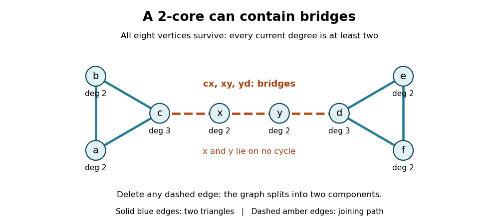
Every vertex of this dumbbell graph survives in the 2-core, including the joining graph path whose three edges are bridges in a graph
. Details. 
Every cycle in a graph does survive pruning, because each of its vertices keeps its two cycle graph neighbours. The barbell shows that the converse fails: the 2-core can be larger than the union of all graph cycles. Its condition is local minimum degree, not protection against a single connection failing.
A biconnected component is a different object: a maximal connected subgraph with no cut vertex of its own. Under the block convention used here, the barbell has five biconnected components: its two triangles and its three individual joining edges, each with its endpoints. Its cut vertices are . A 2-connected component with at least three vertices must remain connected after any single vertex is deleted; the whole barbell fails that test. An informal phrase such as "biconnected core" therefore needs its own definition and must not be substituted for 2-core. Even an isolated edge is a block under this convention, although its 2-core is empty.
The usefulness of the 2-core is this precise separation of local persistence from global robustness. In a connected graph with nonempty 2-core, the deleted vertices form a forest, with each of its connected components of a graph attached by exactly one edge to the 2-core. Otherwise a deleted graph cycle, or a graph path joining two surviving attachment points, would itself have survived. Stripping these attached trees exposes a smaller structure for studying graph cycles, graph excess and the graph kernel, while preserving the joining bridges in a graph that organize that structure.
Suppose is any vertex set whose induced subgraph has every degree of a vertex at least two. No vertex of can be the first one deleted from : before such a deletion it still has its two graph neighbours within , contradicting eligibility for deletion. Consequently every qualifying survives every legal deletion sequence. Once deletion stops, its remainder itself qualifies, because every surviving vertex has at least two surviving graph neighbours. Therefore for every qualifying : is the unique maximum and the final remainder is independent of deletion order. The intermediate FIFO queues and deletion orders can differ.
There is also a direct existence argument. If and qualify, then qualifies: each vertex retains at least the two graph neighbours it already had in or in . Taking the union of all qualifying vertex sets produces the maximum. This rules out a collection of competing, incomparable inclusion-maximal answers. It also explains why restricting the search to connected subgraphs would change the question.
Use adjacency lists and a FIFO queue to implement the deletion rule in time complexity . Compute each initial degree of a vertex once, mark every vertex alive, and put all vertices of degree of a vertex zero or one in the FIFO queue. Each vertex is inserted at most once. Repeatedly remove the front vertex , mark it dead, and traverse its original adjacency list. For each still-alive graph neighbour , decrease the stored degree of a vertex of by one; if it has just become one, append . A vertex already queued can drop from one to zero before its turn, but it stays queued and requires no second insertion. Stop when the FIFO queue is empty; the alive vertices induce .
For the displayed example, initially enqueue in that order. The successive FIFO queues, after each deletion and all its updates, areThis explains the delayed deletion of : its initial degree of a vertex was three, but the relevant degree of a vertex is always its current one in the surviving induced subgraph. Removing only the original vertices of degree of a vertex one would give the wrong answer.
Initialization inspects every vertex and every adjacency list entry once. During deletion each original adjacency list is traversed at most once, so at most entries are inspected in an undirected graph. All insertions, removals and stored-degree updates cost constant time each. Thus total time complexity is and additional storage, beyond the adjacency lists, is . The cost includes isolated vertices; repeatedly rescanning the whole surviving graph after each deletion would lose this bound. The single-threshold FIFO queue method is enough for the 2-core; the full k-core of a graph decomposition computes all thresholds.
A free scalar Klein-Gordon equation with rest mass isHere is the speed of light and the reduced Planck constant. In the static limit, comparison with the static Yukawa Green function identifiesThis is the reduced Compton wavelength, rather than ; the two differ by . It is an exponential decay length of this exchange field, not the geometric size of a nucleon or an exact radius of a bound state. This article uses for a length; the 1935 paper used that letter for its inverse.
For a deliberately rounded worked example, stipulate and . ThenA femtometre is . The chosen rest energy is a convenient pion-scale input; neither it nor the resulting Yukawa potential is asserted to be an exact measured nuclear interaction. Holding fixed, chosen rest energies , and give lengths , and . Doubling the exchange rest mass halves the decay length.
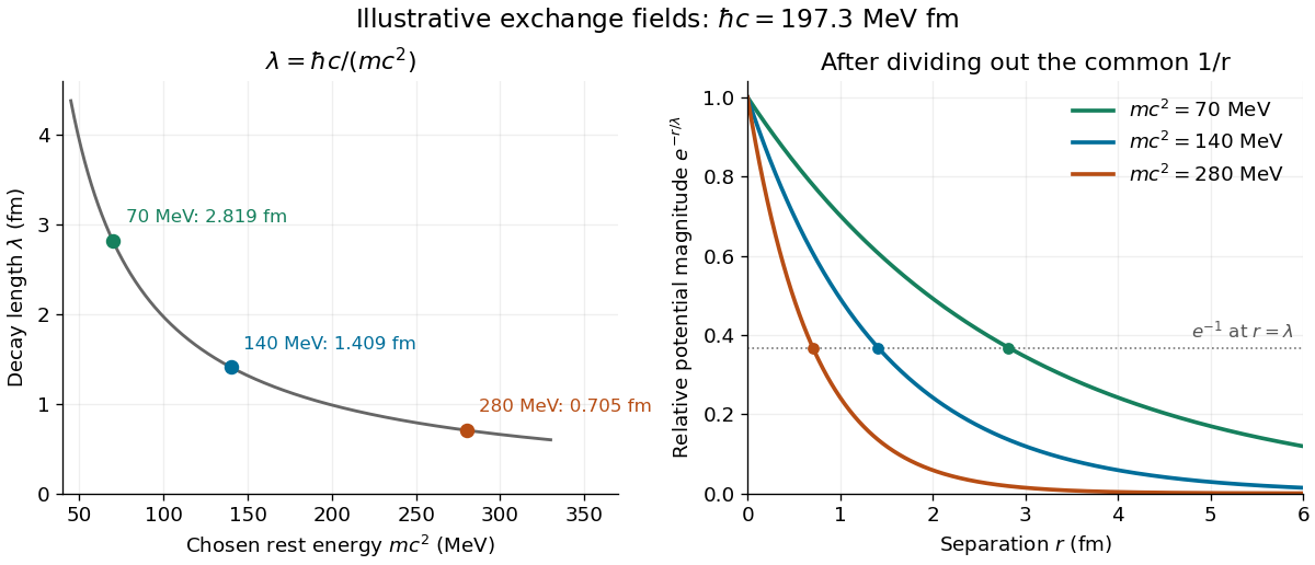

Range alone does not guarantee binding: the potential energy must overcome the kinetic energy cost of localizing a wavefunction. The existing exponential variational bound for the Yukawa potential makes this precise. For the same toy , with reduced mass , choosing a normalized exponential wavefunction proportional to with yieldsFor additional stipulated inputs and , this gives . A negative value proves a bound state in this scalar model by the quantum variational principle; it is an upper bound on its ground-state energy, not a prediction for the deuteron. A nonnegative trial value would not prove the absence of binding.
Let be an inverse length. In three spatial dimensions, seek the Green's function that decays at infinity and satisfieswhere is the Laplacian and the three-dimensional Dirac delta function. The point source and the differential operator have spherical symmetry. For , the radial Laplacian givesWriting reduces this to . Decay at infinity removes the growing exponential function, leaving .
The Dirac delta function fixes the coefficient. Integrating over a ball and using the divergence theorem givesThe first term tends to , while the second is . Hence andThis solves the source equation in the sense of distributions, including at the origin. Merely verifying the equation for would leave the normalization undetermined. The limit at fixed is , the Green function of the Laplacian for the convention .
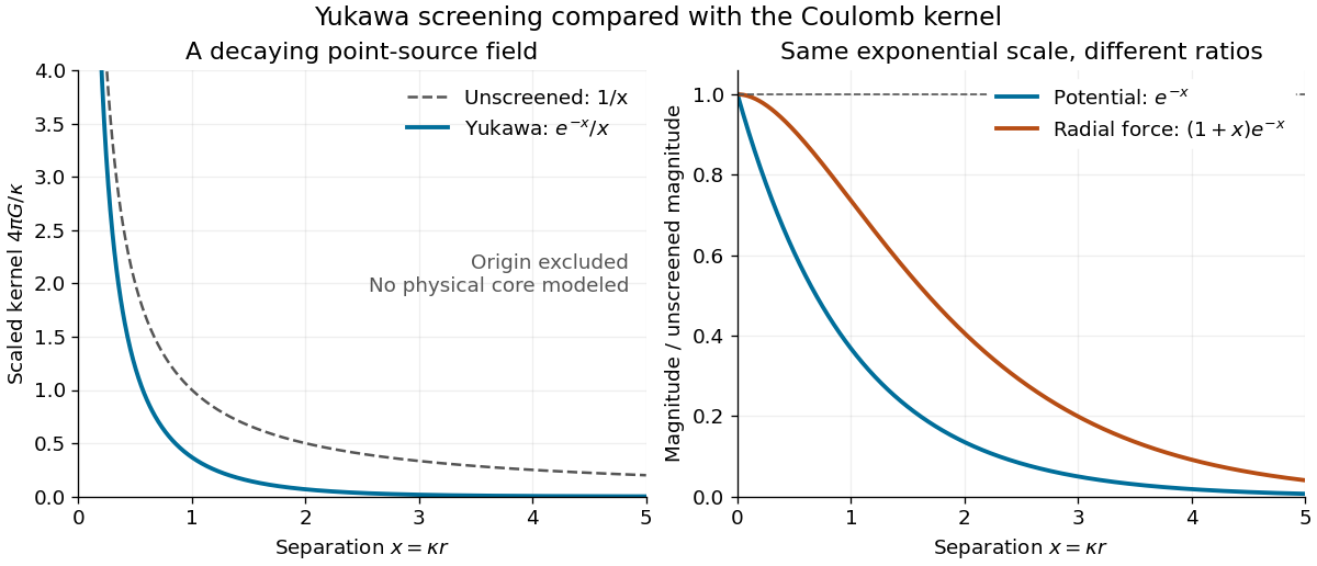
For an attractive scalar toy interaction, absorb constants into and setHere has units of energy times length, and negative points inward. At equal , comparison with the unscreened model givesThus the potential energy and force have the same exponential scale but different suppression factors. At , these ratios are approximately and ; at , they are and . Finite range means rapid decay, not an abrupt cutoff.

There are unlisted articles, also show them or only show them.