Past exam of the astrophysical fluid dynamics course of the University of Cambridge 2021 Section B 5 c Solution by  Codex 0 2026-10-18
The particle count is the enclosed mass divided by the particle mass :Integrating the isothermal Lane-Emden equation giveswhere regularity makes the lower endpoint vanish. ThusThe prefactor is a mass divided by a mass, and the remaining factor is dimensionless. In particular, at fixed the dependence on central mass density is , with . Both changes must be retained when comparing equilibria at fixed .
Past exam of the astrophysical fluid dynamics course of the University of Cambridge 2021 Section B 5 b Solution by Codex 0 2026-10-18
Codex 0 2026-10-18Set and . Then and the equation from part (a) becomesWith , the coefficients cancel, giving the isothermal Lane-Emden equationThe regular central boundary conditions areThe first makes the central mass density equal to . The second follows from smooth spherical symmetry and the vanishing central gravitational acceleration; a preferred radial slope at the origin would be singular. Substitution of a regular power series giveswhich supplies nonsingular starting data for numerical integration. The central conditions select the regular solution, not the singular isothermal sphere.
Past exam of the astrophysical fluid dynamics course of the University of Cambridge 2021 Section B 5 a Solution by Codex 0 2026-10-18
Codex 0 2026-10-18Let be the enclosed mass. For spherical symmetry, hydrostatic equilibrium and mass conservation giveThe isothermal equation of state therefore impliesMultiply by , differentiate and eliminate :or equivalently . This is the density equation for an isothermal sphere. Here has units and equals the squared isothermal sound speed.
A regular isothermal sphere does not reach zero density at a finite radius. The finite body discussed later must therefore be truncated by a nonzero external pressure, as in a pressure-confined isothermal sphere. A finite vacuum boundary would not be compatible with this equation of state.
Past exam of the astrophysical fluid dynamics course of the University of Cambridge 2021 Section B 4 e Solution by Codex 0 2026-10-18
Codex 0 2026-10-18For , , so there is no real solution for an attached straight oblique shock satisfying the assumed geometry. The shock detaches and becomes curved, with a locally strong, nearly normal portion and a subsonic region allowing the flow to adjust to the wall. The precise detached structure depends on the global geometry and downstream conditions; the attached-shock formula cannot be continued to these turns.
Past exam of the astrophysical fluid dynamics course of the University of Cambridge 2021 Section B 4 d Solution by Codex 0 2026-10-18
Codex 0 2026-10-18Rewrite the relation from part (c) asThe angle-addition identities reduce this toFor , the right side lies strictly between zero and one. There are two physically admissible strong oblique-shock angle branches:Both lie between and . They merge when , proving the maximum deflection through a strong perfect-gas shock,For small positive , the formal strong-shock-limit asymptotics areThe weak branch is normally observed for an unconfined supersonic stream turning through a modest compression corner. It has a smaller normal component of upstream velocity, hence a smaller downstream pressure increase; for small turns the downstream flow remains supersonic. The nearly normal strong branch can be selected by suitable downstream pressure conditions, so it is not mathematically forbidden.
The two limits must be ordered honestly. At finite , the weak oblique shock approaches the Mach angle as , rather than zero. The displayed weak-branch asymptotic applies when the large- limit is taken first, or in the overlapping range , where remains valid.
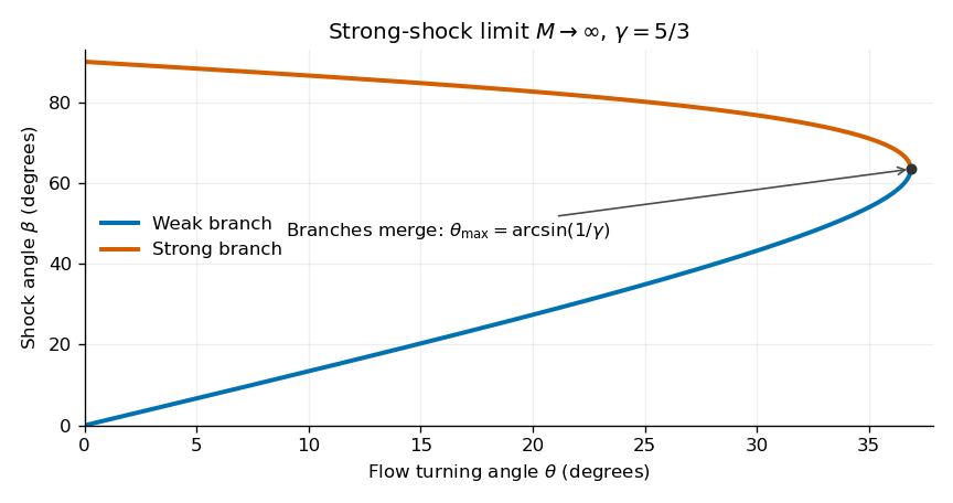
Calculated weak and strong shock-angle branches in the infinite-Mach-number limit, for a monatomic gas
. Details. 
Past exam of the astrophysical fluid dynamics course of the University of Cambridge 2021 Section B 4 c Solution by Codex 0 2026-10-18
Codex 0 2026-10-18Let denote the total flow speeds, keeping the normal components distinct from them. The original diagram measures from the initial wall direction to the shock wave itself. The outgoing velocity is turned by , so it makes angle with the shock.
Resolve each velocity tangent and normal to the oblique shock. Tangential momentum conservation, with nonzero mass flux and no tangential surface force, makes the tangential velocity continuous:The normal flow obeys the strong normal shock wave result from part (b):Divide the second relation by the first to obtainThe approximation is controlled by the upstream normal Mach number , not just by . This distinction matters on the small-angle weak branch in part (d). The angle convention is also important: formulas using the angle to the shock normal instead would interchange sine and cosine.
Past exam of the astrophysical fluid dynamics course of the University of Cambridge 2021 Section B 4 b Solution by Codex 0 2026-10-18
Codex 0 2026-10-18Take . Let . Mass conservation gives , and normal momentum conservation givesInsert this into the energy condition from part (a):Rearranging and factoring,The root is the unshocked state. The compressive Strong-shock Rankine-Hugoniot conditions instead giveCorrespondingly, and . These relations require and negligible upstream thermal pressure.
Past exam of the astrophysical fluid dynamics course of the University of Cambridge 2021 Section B 4 a Solution by Codex 0 2026-10-18
Codex 0 2026-10-18A shock wave forms when a compressive flow steepens or when gas must be decelerated or turned faster than upstream acoustic waves can communicate the change. Astrophysical examples include a supernova remnant sweeping up surrounding gas, a fast stellar wind colliding with ambient material, and supersonic accretion onto an obstacle or onto a dense gas layer. A large Mach number by itself is not sufficient: a uniform supersonic stream need not contain a shock wave.
Choose the shock frame, and denote upstream and downstream normal velocities by . Integrating the local conservation laws over a thin control volume spanning a steady normal shock wave gives equal fluxes on both sides. Mass conservation gives constant mass flux per unit area,Pressure and advected momentum together give the normal momentum flux,For a thin non-radiating layer, with negligible gravitational-potential change across it, conservation of energy gives equal fluxes . A perfect gas has specific enthalpy , soThese are the Rankine-Hugoniot conditions for a perfect gas. Dissipation inside the thin layer produces an entropy increase and selects the physical compressive branch. Efficient radiative cooling would change the energy relation and may instead lead to an isothermal shock.
Past exam of the astrophysical fluid dynamics course of the University of Cambridge 2018 Section A A1 c Solution by Codex 0 2026-10-18
Codex 0 2026-10-18For a plane-parallel slab, all equilibrium quantities depend only on height . The vertical hydrostatic equilibrium equation and the Poisson equation for Newtonian gravity areWith the polytropic equation of state and constant ,In the gas interior, where , divide by and differentiate once:ConsequentlyThe coefficient has units inverse square metres. The index-one plane-parallel polytrope illustrates the resulting structure: symmetry about gives , with . A slab bounded by vacuum ends at its first zero, ; the negative continuation of the cosine is not physical mass density.
Past exam of the astrophysical fluid dynamics course of the University of Cambridge 2018 Section A A1 b Solution by Codex 0 2026-10-18
Codex 0 2026-10-18Use the nonrelativistic moving-conductor Ohm law in the formThe Maxwell equations give Faraday's law of induction, . For a nonmagnetic conductor with constant permeability , the quasistatic Ampere-Maxwell law gives . This step neglects displacement current, requiring it to be small compared with conduction current; nonrelativistic velocity alone is not the complete justification.
For spatially uniform scalar electrical conductivity ,Apply the identity and Gauss's law for magnetism, . The resistive induction equation isThe first term transports and deforms the magnetic field with the moving fluid; the second diffuses it. The magnetic diffusivity has units , so both terms have units tesla per second. No assumption of incompressible flow was needed. If varies spatially, the conductivity-gradient term in magnetic induction, , must also be retained.
Past exam of the astrophysical fluid dynamics course of the University of Cambridge 2018 Section A A1 a Solution by Codex 0 2026-10-18
Codex 0 2026-10-18Take positive to mean net removal of thermal energy per unit mass. The isobaric thermal stability of a heated ideal gas depends on the density change accompanying a temperature disturbance. For an ideal gas of fixed composition, , so constant pressure gives . Therefore the net cooling can be writtenwhere is constant for this pressure. At thermal equilibrium , .
The first law of thermodynamics at constant pressure includes the expansion work, so the relevant heat capacity is the specific heat capacity at constant pressure, , rather than the constant-volume value. Linearizing its temperature equation givesHenceFor optically thin Bremsstrahlung, , soA hotter parcel expands and becomes less dense. Its cooling per unit mass, proportional to at fixed pressure, decreases while its cosmic ray heating stays fixed, making it hotter still. A colder, denser parcel cools faster and runs away in the opposite direction. Here has units and units , so is an inverse time. The conclusion assumes the disturbance remains close to pressure equilibrium and neglects heat conduction and changes of composition. The relevant is the temperature exponent in the supplied cooling law.
Past exam of the advanced quantum physics course of the University of Cambridge 2022 Section B 6 e Solution by Codex 0 2026-10-18
Codex 0 2026-10-18The thermal oscillator occupation is the Bose-Einstein distribution. With the rate notation for a transition from to , the master equation for the up population isAt thermal equilibrium, assuming , vanishing time derivative is detailed balance between the two spin states. HenceorTogether with normalization, this gives and , the Boltzmann distribution for the energy eigenvalues . At zero temperature, absorption vanishes and emission relaxes the spin into its down ground state.
The nonzero-rate condition is necessary: if or , both rates vanish, so every initial pair of populations is stationary within this approximation. In that case stationarity alone cannot imply a thermal distribution. The equilibrium conclusion therefore presumes coupling to resonant oscillator modes.
Past exam of the advanced quantum physics course of the University of Cambridge 2022 Section B 6 d Solution by Codex 0 2026-10-18
Codex 0 2026-10-18In first-order time-dependent perturbation theory, the resonant time factor before taking the Fermi's golden rule limit isIts central frequency width is of order , and its total area is . To replace it by , the oscillator density of states and relevant occupations must be approximately constant over that width. Thus . At the same time, the perturbative flip probability must remain much smaller than one.
Define , so the two flip rates are and . A sufficient common time window for both initial spins isFor a specified initial spin, the upper condition is simply its own flip rate times . Such a window requires weak enough coupling. The continuum approximation also presumes times shorter than recurrences from a resolved finite oscillator spectrum, and long enough to resolve the positive-frequency resonance from its nonresonant counterpart.
Past exam of the advanced quantum physics course of the University of Cambridge 2022 Section B 6 c Solution by Codex 0 2026-10-18
Codex 0 2026-10-18The Pauli matrix flips the spin with unit matrix element. A nonzero oscillator matrix element changes exactly one occupation number, through a creation operator or an annihilation operator:For a spin flip, the spin energy change divided by is . Thus creation and annihilation in mode have total frequency changes and , respectively. Distinct modes or different occupation changes lead to orthogonal final quantum states, so their probabilities add. Fermi's golden rule consequently givesThe Dirac delta function is even, accounting for the sign in the annihilation term. Since all , an initially up spin can only emit an oscillator quantum, while an initially down spin can only absorb one. Writing the oscillator density of states per unit angular frequency as , the continuum limit givesThe permits emission even from the oscillator vacuum; absorption requires a quantum already present. The notation assumes a common or smoothly specified occupation at the resonant frequency. If several resonant modes have different occupations, it denotes their density of states weighted mean, so that after continuum smoothing. This is the golden-rule relaxation of a spin coupled to an oscillator bath.
Past exam of the advanced quantum physics course of the University of Cambridge 2022 Section B 6 b Solution by Codex 0 2026-10-18
Codex 0 2026-10-18The orthogonal projection onto the full spin- subspace isHere the identity acts on all oscillator states. The finite-time scattering operator in the question is the interaction picture time-evolution operator, so . Projecting its two orthogonal spin components yieldsExpand the right-hand side in the orthonormal basis . Taking its squared norm, and using the normalization of , givesThus one sums probabilities over unobserved final oscillator states, not their probability amplitudes. Unitarity of makes the sum over both equal to one.
Past exam of the advanced quantum physics course of the University of Cambridge 2022 Section B 6 a Solution by Codex 0 2026-10-18
Codex 0 2026-10-18For this spin-boson model, take . Since , the interaction picture observable isThe normalized vectors and belong to different eigenspaces of the Hermitian operator , and are therefore orthogonal. This remains true even though each vector includes the oscillator degrees of freedom. Hence all cross terms in the expectation value vanish, while the diagonal terms have eigenvalues and :Normalization also gives , so these are the probabilities of the two spin outcomes.
Past exam of the advanced quantum physics course of the University of Cambridge 2022 Section B 5 d Solution by Codex 0 2026-10-18
Codex 0 2026-10-18Normalize the trial quantum state as . With the phases used above, the off-diagonal position matrix element is . DefineThe diagonal perturbation matrix elements vanish by parity, so the Rayleigh quotient isThe stationarity equation is . The minimum continuously connected to the unperturbed ground energy eigenstate hasEquivalently, diagonalize the Hamiltonian operator matrix in this two-dimensional trial space. Its lower eigenvalue isThereforeThis retains exactly the term of the full ground-state second-order nondegenerate perturbation theory sum. Every omitted term is negative, so the full quadratic correction is more negative than this restricted one. This is consistent with the Rayleigh-Ritz variational principle: minimizing over a two-state subspace gives an upper bound on the exact ground energy. The bound applies to the unexpanded two-state minimum; a truncated series is to be compared order by order.
Past exam of the advanced quantum physics course of the University of Cambridge 2022 Section B 5 c Solution by Codex 0 2026-10-18
Codex 0 2026-10-18The electron's electric dipole moment is . It vanishes in the unperturbed ground energy eigenstate. The first correction to the wavefunction is linear in the electric field and has the opposite parity; its interference with the unperturbed state therefore gives a nonzero position expectation value of first order.
In detail, the normalized ground quantum state, to the order needed, isThe normalization correction starts at second order and does not affect the linear term below. The two cross terms giveThe absence of an term follows from the parity operator: changes sign under field reversal. Comparing with the second-order nondegenerate perturbation theory energy sum yieldsThus the induced electric dipole moment points along the electric field, with positive electric polarizability. The induced dipole moment and quadratic energy shift obey . This factor of one half accounts for the energy needed to induce the dipole. As a check, the Hellmann–Feynman theorem gives , with the same result.
Past exam of the advanced quantum physics course of the University of Cambridge 2022 Section B 5 b Solution by Codex 0 2026-10-18
Codex 0 2026-10-18Use zero-based labels to agree with in the later parts. The normalized infinite square well energy eigenstates and energy eigenvalues areThe position matrix elements in a symmetric infinite square well, obtained by integrating the product of the two wavefunctions against , areThe integral in the question uses positive integer labels; replacing them by is essential here. Only opposite-parity states, odd, contribute, as also follows from the parity operator selection rule.
Second-order nondegenerate perturbation theory now gives the requested infinite sum:In fully explicit form this isThe symbol here denotes the electron mass, not a summation index. For the ground state , every denominator in the first form is negative, so the ground energy level moves downward. For excited states, contributions from lower and higher energy levels have opposite signs.
Past exam of the advanced quantum physics course of the University of Cambridge 2022 Section B 5 a Solution by Codex 0 2026-10-18
Codex 0 2026-10-18The unperturbed infinite square well is invariant under the parity operator. Its one-dimensional energy eigenvalues are nondegenerate, so each energy eigenstate has definite parity. Its position expectation value therefore vanishes: is even, while is odd. The first-order nondegenerate perturbation theory correction is consequentlyThe electric field does mix opposite-parity quantum states, and second-order nondegenerate perturbation theory contains two factors of . Its leading contribution is thus proportional to : this is a quadratic Stark effect. More generally, applying the parity operator changes into , so their corresponding energy eigenvalues agree. An analytic expansion about zero electric field contains only even powers of . We assume is small compared with the unperturbed excitation scale.
There are unlisted articles, also show them or only show them.