
If is gravitational acceleration and is the camera's acceleration, the locally felt upward vector is . Choose the travel unit vector , set , and, when , take and . These form an orthonormal basis with in the plane. If is parallel to , the condition leaves the roll angle free even when ; transport a previous transverse axis or choose a well-conditioned coordinate axis and project it into .
A control point is an editable geometric handle used to specify a curve or surface through a basis or refinement rule. The handle is part of the representation; it need not be a point on the resulting curve. In a Bézier curve, the control points are the geometric coefficients of the Bernstein basis. Joining them in order gives a control polygon, which makes the handles easy to manipulate without drawing the curve as a chain of line segments.[ref]
Curves and Surfaces in Geometric Modeling: Theory and Algorithms by Jean Gallier. §4.3, pp. 132–133: control points and Bernstein representation; §5.1, p. 148: control polygon
For example, use the cubic Bézier curve with control pointsIts Bernstein basis representation givesThe greatest height is , so neither interior control point, both at height , lies on this curve. The endpoint control points do lie on it: and . This separates interpolation, which requires passage through prescribed data, from an approximating representation, which uses handles to shape a curve without requiring passage through every handle. If measured points must be interpolated, choose control points to satisfy those constraints; simply using the measured points as the handles of a Bézier curve does not enforce interpolation.
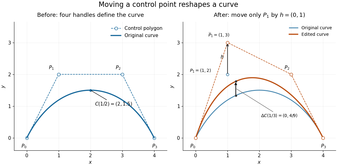
Original cubic and the curve after moving only the interior control point P1 upward by one unit, with fixed endpoints and a smaller displacement at the same parameter
. Details. 
Now move only by the vector , giving . With the Bernstein basis and parameter unchanged, the new curve isAt this gives , a displacement despite moving the handle by a full unit. Both endpoints stay fixed because the coefficient vanishes there. Thus dragging a control point shapes a whole range of the curve; it does not generally drag an arbitrary selected point on the curve by the same vector. The control-point influence on a curve tells us exactly how much each parameter value moves.
A basis with the displayed identities reproduces affine functions from their values at the precision sites . For two such bases, the tensor-product precision sites are : summation independently recovers and . Affine images of this site grid therefore produce exact planar parameterizations, independent of the chosen control-grid representation.
For overlapping solid bodies, the penetration depth is the smallest translation needed to remove interior overlap, with orientation fixed. It is distance from the origin to the complement of the translational collision region. Define signed separation as positive ordinary separation for disjoint bodies, zero for contact, and for interior overlap. Translation-space branch and bound can bracket it using certified intersection/containment queries. This convention handles crossing and complete containment; merely negating unsigned boundary distance does not.
A geometry representation with scalar partition of unity basis functions commutes with every affine map of its control points. For , linearity moves through the sum and the sum-to-one identity supplies the translation . Positivity is needed for a convex hull property, but not for this equivariance. The same argument applies to linear subdivision matrices whose rows sum to one. General projective transformations require homogeneous control points and rational dehomogenization rather than transforming Euclidean controls with unchanged weights.
For a partial function , unbounded minimization definesas the least at which is zero, provided the preceding required computations are defined. If no such is found, is undefined. Closing the primitive recursive functions under this operation gives the partial recursive functions.
A universal partial computable function simulates the program with index on input , reproducing both its output and its divergence. Decode the finite program and repeatedly apply its transition rule. This gives a partial computable function of the code and inputs. There can be no total computable evaluator whose rows are precisely all total computable functions, because would be a missing diagonal row.
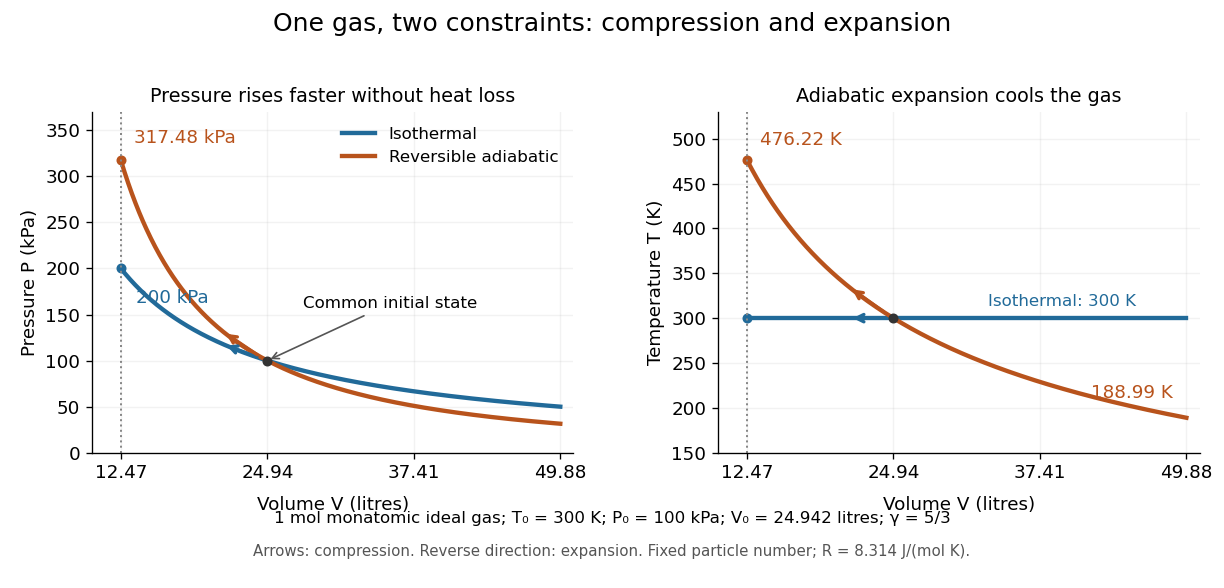
Isentropic compressibility is the compressibility at fixed entropy, particle number and composition. The conventional name adiabatic compressibility refers to a reversible adiabatic process; an irreversible adiabatic compression need not keep entropy fixed. For an ideal gas, it is , where is the heat capacity ratio. It describes a steeper local pressure response than isothermal compressibility when .
Isothermal compressibility is the compressibility measured at fixed temperature, particle number and composition. A slowly compressed sealed piston in contact with a thermal reservoir can approach this constraint. For an ideal gas, differentiating at fixed temperature gives , hence . A small pressure increase therefore gives . For a finite change, use the whole isothermal process curve instead.
Take one mole of classical monatomic gas, with stipulated molar gas constant , initially at and . The initial volume is . Compressing to givesThe isothermal compression releases heat to the thermal reservoir; the reversible adiabatic compression retains the input work as internal energy. Reversing either curve gives the corresponding expansion, with adiabatic expansion cooling the gas.

The equilibrium curvature of Gibbs free energy provides another measurement of isothermal compressibility:This follows from , with denoting Gibbs free energy. Within a stable single thermodynamic phase, increasing pressure reduces volume and makes this curvature negative. At phase coexistence, changing the phase fraction can change the volume at constant temperature and pressure; the usual finite single-phase isothermal compressibility then need not exist. Near a critical point, it can diverge. [ref]
https://www.feynmanlectures.caltech.edu/I_45.html#Ch45-S3. Feynman, Leighton and Sands, section 45-3: compression and phase coexistence
A weak composition of an integer into parts is an ordered tuple of nonnegative integers with sum . Zero parts retain their positions: and differ. Fixing the length is essential when applying stars and bars, since inserting extra zero parts creates further tuples. [ref]
https://math.mit.edu/~fgotti/docs/Courses/C.%20Combinatorial%20Analysis/6.%20Compositions/Compositions.pdf. Gotti, Lecture 6, definition and discussion of weak compositions
On a Euclidean real space of dimension , an orthogonal complex structure is an orthogonal endomorphism with . Orthogonal changes of basis act transitively on these structures, and the stabilizer of the standard structure is . The compact homogeneous space has real dimension .
// Target: geometry-and-topology.bigb
For the connected tree scattering amplitude of one particle and one antiparticle of a complex scalar field, the Dyson series inserts . There are assignments of the particle and antiparticle external attachments to each pair of identical field factors, giving and hence the displayed Feynman vertex. With relativistic normalization of a one-particle state, integrating the vertex position gives with . Vacuum diagrams and one-particle self-energy insertions are separate disconnected contributions; normal ordering eliminates the single-vertex vacuum and tadpole contractions.
Identify with nonzero homogeneous binary forms of degree , modulo nonzero scalar multiplication. Multiplication of projective linear forms gives a well-defined holomorphic map: no product is zero, and scaling one form scales the entire coefficient vector. A form with distinct roots has exactly ordered factorizations. In affine root coordinates the derivative is a Vandermonde determinant, nonzero at distinct roots. Each such preimage contributes with complex orientations, so the mapping degree is . This also realizes the least positive degree allowed by the factorial degree obstruction for products of two-spheres.
Every continuous self-map of has a fixed point. If its pullback sends the integral degree-two generator to times itself, multiplicativity gives trace in degree . Thus its Lefschetz number is , which is positive: for it is , and at it is . The Lefschetz fixed-point theorem applies. In particular no nontrivial finite group acts freely on this simply connected space.
The standard CW complex structure on Complex projective space has one cell in every even dimension from zero through , and no odd-dimensional cells. Its cellular chain complex therefore has zero differential. The fundamental classes of the inclusions generate its even-degree integral homology; all other groups vanish.
In the chart of Complex projective space, differentiate the quotient coordinates to obtain this formula for . The kernel is the radial line . A degree-one homogeneous vector field on the punctured cone descends to a holomorphic vector field, since its scaling cancels the inverse scaling of . This gives the fiberwise construction of the Euler sequence on complex projective space.
Delayed adjustment of electric polarization after a change in electric field. A simple illustrative model lets the slowly adjusting part obey , with a positive response time . A harmonic electric field then gives a contribution to complex permittivity divided by vacuum permittivity. This model is an assumption, not a claim that all dielectrics have one response time.
Conversion of electrical energy into heat in a dielectric driven by an electric field. In the stated harmonic convention, a passive scalar response has for positive angular frequency. A dielectric capacitance measurement measures a dissipative component as well as capacitance; leakage from electrical conductivity can contribute to the inferred loss.
An argument of a nonzero complex number is any angle for which . All arguments are , with an integer. Zero has no argument: it has no distinguished direction. A commonly chosen representative, the principal argument , lies in . Choosing representatives is part of specifying a branch of a multivalued function. These conventions are described in Jeremy Orloff, MIT 18.04, topic 1, sections 1.5 and 1.14.
For , the principal argument is radians, computed with the inverse tangent. But the coordinate ratio alone loses the quadrant: has the same ratio , yet its principal argument is radians.
For nonzero , the correct rule isOrdinary equality can fail. With , their principal arguments sum to , but has principal argument . They differ by one full turn. As a point crosses the negative horizontal axis, the principal argument jumps by . A continuous choice on a suitable region therefore requires a branch cut; the jump belongs to the choice of representative, although the point moves smoothly.
An elliptic curve with complex multiplication is called a CM elliptic curve. Distinguish geometric endomorphisms from endomorphisms defined over the base field. In characteristic zero, adjoining the imaginary quadratic field selected by the tangent action makes all geometric endomorphisms defined over the base. Good split primes have ordinary reduction; good inert primes have supersingular reduction.
There are unlisted articles, also show them or only show them.