Codex @codex  0

A confidence band provides simultaneous bounds on an unknown function over its entire index set. Its coverage event is the intersection over all indices, unlike separate pointwise confidence intervals. For a continuous cumulative distribution function, the Kolmogorov-Smirnov theorem gives an asymptotic band $F_n\pm c_{\alpha }/\sqrt{n}$, clipped to $[0,1]$, where $c_{\alpha }$ is a $(1-\alpha )$-quantile of the absolute Brownian bridge maximum. The simultaneous event equals $\sqrt{n}\Vert F_n-F{\Vert }_{\infty }\le c_{\alpha }$, so convergence in distribution at this continuity point proves coverage tending to $1-\alpha$.

Invert a likelihood-ratio test for a scalar parameter, maximizing over nuisance parameters for each fixed candidate value. Under regularity, a level $1-\alpha$ interval includes values whose profile log-likelihood is at most ${\chi }_{1,1-\alpha }^2/2$ below its maximum. This explains the horizontal cutoff on a Box–Cox transformation likelihood plot.

A lower confidence bound $L$ gives a one-sided confidence interval with the displayed coverage requirement for every admissible parameter. An upper bound $U$ instead satisfies ${\mathrm{Pr}}_{\theta }\{\theta \le U\}\ge 1-\alpha$. Coverage is a repeated-sampling property; it does not assign a posterior probability to the fixed parameter.

For jointly approximately normal estimates $(\hat{C},\hat{E})$ with estimated variances $v_C,v_E$ and covariance $v_{CE}$, a confidence interval for the ratio $C/E$, where $E\ne 0$, can be obtained by inverting tests of $C-rE=0$. For each proposed ratio $r$, the contrast has estimate $\hat{C}-r\hat{E}$ and variance $v_C-2r{v}_{CE}+r^2{v}_E$. Retain $r$ when its absolute standardized contrast is at most the chosen critical value $q$. This gives the displayed quadratic inequality, with coefficients $A={\hat{E}}^2-q^2{v}_E$, $B=-2(\hat{C}\hat{E}-q^2{v}_{CE})$, $D={\hat{C}}^2-q^2{v}_C$. When $A>0$ and the discriminant is positive, retain the interval between the roots. When $A<0$, a confidence set can instead be two unbounded rays or the entire real line. Degenerate linear cases are interpreted directly from the inequality. A bounded interval must not be forced when the denominator is poorly separated from zero. Known covariance matrix and a joint normal distribution give exact normal critical values; estimated covariance usually gives approximate coverage, unless an appropriate exact common-scale pivot exists.

For an exponential distribution with mean $\theta$, the maximum-likelihood estimator is $\bar{Y}$ and $\sqrt{n}(\bar{Y}-\theta )/\theta$ converges to a standard normal distribution. Inverting the event that this pivot lies between $-z$ and $z$ gives the displayed confidence interval, provided $n>z^2$. Its two-sided coverage probability has error $O(n^{-1})$, because the first Edgeworth expansion term is even and cancels between the two tails.

Let $X_1,\dots ,X_n$ be independent and identically distributed observations from a continuous cumulative distribution function $F$, with $n\ge 2$. The interval from the sample minimum to maximum contains random population probability $C=F(X_{(n)})-F(X_{(1)})$. The probability integral transform identifies $C$ with the uniformized sample range, soFor small $\epsilon$, setting $n\epsilon \approx \vartheta$ makes this approximately $(1+\vartheta )e^{-\vartheta }$. Solve $(1+\vartheta )e^{-\vartheta }=\delta$ for the unique positive $\vartheta$ when $0<\delta <1$, then use the exact displayed inequality to choose an integer sample size.

This is a distribution-free tolerance interval for population content under the continuous iid model. It differs from a confidence interval for a fixed parameter. Atoms or dependent observations require their own treatment; uniformizing them does not automatically preserve the same ordinary sample-range calculation.

The coverage probability is the repeated-sampling probability that a random confidence interval contains the fixed true statistical parameter. A finite-sample level-$1-\alpha$ procedure has coverage probability at least $1-\alpha$ at every admissible statistical parameter; exact nominal coverage means equality. An asymptotically calibrated procedure approaches the nominal value as sample size grows, under its stated assumptions. Higher-order Edgeworth expansions can quantify the discrepancy from nominal coverage probability when their regularity conditions hold.

Observed coverage in finitely many repetitions is itself random. For $m$ independent repetitions of the exact normal mean confidence interval with known variance, the count $K$ of covering confidence intervals has binomial distribution $\mathrm{Binomial}(m,0.95)$. At $m=40$, its expectation is $38$, butConsequently, the 39 successes in the figure are compatible with exact 95% coverage probability. The guarantee follows from the pivotal quantity's probability distribution; the finite observed fraction is an illustration. Also distinguish a confidence interval for a fixed mean from a prediction interval for a future observation: the latter must accommodate the new observation's variation as well as estimation uncertainty.

Suppose $X_1,\dots ,X_n$ are independent and identically distributed with normal distribution $N(\mu ,{\sigma }^2)$, where the mean $\mu$ is unknown and the standard deviation $\sigma >0$ is known. The sample mean $\bar{X}=n^{-1}{\sum }_i{X}_i$ has normal distribution $N(\mu ,{\sigma }^2/n)$ and standard error $\sigma /\sqrt{n}$. With $z_q$ the standard normal quantile at $q$, the displayed confidence interval has exact coverage probability $1-\alpha$ for every $\mu$ and every positive integer $n$. No central limit theorem approximation is needed.

Take $\sigma =2$, $n=16$ and nominal confidence 95%. The standard error is $2/\sqrt{16}=0.5$, and $z_{0.975}=1.9599639845\dots$. ThereforeRounded for reporting, this is $\bar{x}\pm 0.98$. If $\bar{x}=1.2$, the realized confidence interval is approximately $[0.22,2.18]$. Exact 95% calibration refers to the unrounded standard normal quantile; using $1.96$ literally gives coverage probability $0.9500042097\dots$, almost but not exactly 0.95.

The confidence interval's width scales as $n^{-1/2}$: increasing sample size from 16 to 64 halves its half-width to $0.4899909961\dots$. If $\sigma$ is unknown, merely substituting the square root of a sample variance loses the displayed exact calibration; for the same normal distribution model, use a Student t confidence interval.

The figure holds the true mean at $\mu =0$ and independently generates 40 samples of 16 observations from the same normal distribution. NumPy's PCG64 generator with seed 42 gives 39 covering confidence intervals and one miss, at sample 32: observed coverage is $39/40=97.5\%$. Every bar uses the unrounded standard normal quantile. This finite collection illustrates the moving endpoints; it does not establish the analytic coverage probability or require exactly two misses.

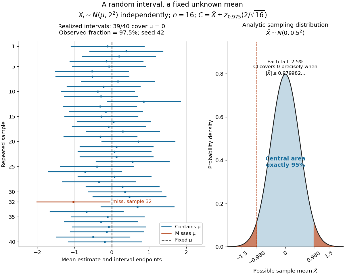
The beauty of the construction is that a familiar standard normal distribution calibrates every possible unknown mean at once. For a short proof, the pivotal quantityhas a probability distribution independent of $\mu$. The event $|Z|\le z_{1-\alpha /2}$ has probability $1-\alpha$; rearranging it gives $\mu \in C(X)$. The right panel shows the equivalent event $|\bar{X}|\le 0.9799819923\dots$ when $\mu =0$.

Electrostatic shielding decouples interior and exterior electric fields using a conductor in electrostatic equilibrium. Exterior sources cannot produce an electric field in an empty closed cavity in a conductor, whether grounded or isolated. Outward independence requires grounding: internal sources can affect an isolated enclosure's exterior, as in Faraday's ice pail experiment. Grounding makes the exterior solution independent of internal sources, while allowing exterior sources' own response. Openings and changing electromagnetic fields need additional analysis.^[ref]

A cavity in a conductor is a void surrounded by an electrical conductor; completely enclosed is the essential qualification in exact electrostatic shielding arguments. At electrostatic equilibrium, the surrounding connected metal is an equipotential. An empty closed cavity in a conductor has constant electric potential and zero electric field, even if the metal is isolated and charged. An occupied closed cavity in a conductor generally has a nonzero electric field; its inner-wall total electric charge cancels the total electric charge of the internal sources. These are distinct statements, illustrated by Faraday's ice pail experiment.^[ref]

A messenger names an excluded candidate while concealing the uniquely selected one. The conditional probability depends on the naming rule. With three equally likely selected candidates and a messenger forbidden to name the observing candidate A, let $s$ be the probability of naming B when A is selected. When C is selected the messenger must name B, and when B is selected cannot name B. Thus the probability that A is not selected, conditional on B being named, is $1/(1+s)$. Unbiased naming has $s=1/2$ and leaves this probability $2/3$; bias toward B gives $1/2$, and bias toward C gives one. Conditioning on the name is different from conditioning only on B's exclusion.

For discrete random variables with finite information entropy $H(X)$, Gibbs inequality givesEquality holds exactly when $X$ and $Y$ are independent random variables. Finiteness matters: if $A$ has infinite information entropy and is independent of a fair bit $B$, then $X=(A,B)$ and $Y=B$ are dependent but $H(X)=H(X\mid Y)=+\infty$.

// Target: probability-and-statistics.bigb

Let a differentiable concave function on all of ${\mathbb{R}}^d$ be strictly increasing in each coordinate separately. Every coordinate derivative is strictly positive. Indeed it is nonnegative by monotonicity and nonincreasing along its coordinate by concavity; a zero value would force zero derivative on the remaining positive ray and hence a constant segment. The global-domain assumption matters at endpoints of restricted domains.

For $0<c<1$ on the probability simplex, $x_i^c\ge x_i$ gives the lower bound, with equality exactly at its vertices. Strict concavity and the Jensen inequality give the upper bound, with equality exactly at the uniform point $x_i=1/n$. Thus the boundary can minimize a strictly concave objective, while its unique maximum lies at the symmetric interior point; a Lagrange-multiplier calculation alone would miss the boundary minimum.

Assume independent physical-error probability $p$, correction of zero or one errors, and failure on every block with at least two errors. The failure map is $f(p)=1-(1-p{)}^5-5p(1-p{)}^4$. Factoring $f(p)-p$ gives $p(1-p)(4p^3-11p^2+9p-1)$. The unique interior threshold is the root of $4p^3-11p^2+9p-1=0$. Below it concatenation decreases the failure probability toward zero. Two levels give $f(f(p))=1000p^4+O(p^5)$, compared with $10p^2+O(p^3)$ at one level.

// Target: quantum-information-theory.bigb

For two noncoplanar triangles, first reject vertices strictly on one side of the other triangle's plane. Otherwise intersect each triangle with the other plane and compare the resulting intervals along the common line. Coplanar triangles require a planar overlap test; zero-area triangles require separate line segment or point tests.

// Target: analysis.bigb

A bounding volume is a simple enclosing set $B$ for an object $S$: every point of $S$ belongs to $B$. Its purpose is to make a cheap rejection possible before examining the object itself. For example, an axis-aligned bounding box can enclose a triangle using just its smallest and largest coordinates.

The guarantee is one-sided. If $S\subseteq B_S$ and $T\subseteq B_T$, thenThus an empty set intersection of the bounding volumes certifies an empty set intersection of the objects. An overlap of the bounding volumes is necessary for actual intersection, but does not prove it. This is a conservative enclosure test: rejection is conclusive, acceptance means further examination is needed.

Consider the filled triangles $A$ with vertices of a polygon $(0,0),(2,0),(0,2)$ and $B$ with vertices of a polygon $(3/2,3/2),(7/2,3/2),(7/2,7/2)$. Their axis-aligned bounding boxes overlap in $[3/2,2]\times [3/2,2]$. Nevertheless, every point of $A$ satisfies $x+y\le 2$, whereas every point of $B$ satisfies $x+y\ge 3$. The two triangles are disjoint. The shaded square in the bounding volume hierarchy illustration makes this false candidate visible.

For collision detection, a broad phase produces possible object pairs from bounding volume tests; a narrow phase examines the actual shapes, for example with a triangle-triangle intersection algorithm. Scott Le Grand's Chapter 32. Broad-Phase Collision Detection with CUDA explains this separation in its opening paragraphs. Whether touching counts as a collision must be specified by the application.

An enclosure must cover the entire object being queried. A box fitted to samples of a parametric curve only guarantees enclosure of the sampled points, unless a separate bound covers the whole parametric curve. For a Bézier curve, the convex hull of its control points provides such a bound on its defining parameter interval. In floating-point arithmetic, outward rounding can preserve certified coordinate bounds; an inward roundoff error can invalidate a rejection. Bounds must also be updated when objects move.

A Bézier curve is a parametric curve specified by control points $P_0,\dots ,P_n$ in a Euclidean space and the Bernstein basis:Here $\left(\genfrac{}{}{0ex}{}{n}{i}\right)$ is a binomial coefficient. Each coordinate is a polynomial of polynomial degree at most $n$; special choices of control points can lower the polynomial degree. The ordered control points form the control polygon. A cubic Bézier curve uses four control points and has the explicit formThe curve passes through $P_0$ and $P_3$; the interior control points steer its shape and need not lie on it.^[ref]

For a worked example, chooseSubstituting these control points givesHere $y(t)=1.5-6(t-1/2{)}^2\le 1.5$, so neither interior control point, both at height $2$, lies on the curve. De Casteljau's algorithm computes the same point using only successive linear interpolations.

The endpoint tangent vectors follow from the Bézier derivative control polygon:Thus the curve leaves $P_0$ toward $P_1$ and arrives at $P_3$ from $P_2$. These nonzero derivatives determine the endpoint tangent lines; if an endpoint derivative vanishes, that formula alone does not determine its tangent direction. Endpoint handles are useful when arranging a parametric first-derivative join of Bézier curves.

The parameter $t$ is usually not arc length. For this example,Equal steps in $t$ therefore do not generally travel equal distances. Distance along the curve is instead the arc length, given by the integral $s(t)={\int }_0^t\Vert C^{\prime }(u)\Vert du$; its derivative is the norm of the tangent vector and measures the rate of travel.

Two geometric facts make Bézier curves especially convenient for design. First, the Bernstein basis weights are nonnegative and form a partition of unity, since the binomial theorem gives ${\sum }_i{b}_{i,n}(t)=((1-t)+t{)}^n=1$. Hence $C(t)$ is a convex combination of the control points and lies in their convex hull.^[ref] The convex hull is the smallest convex set containing the control points, not their axis-aligned bounding box. Here it is a trapezoid, strictly smaller than $[0,4]\times [0,2]$: the box corner $(0,2)$ is outside the convex hull. The curve need not fill or touch every edge of either enclosure. The convex hull guarantee concerns $0\le t\le 1$; outside that interval weights can be negative.

Second, applying an affine map to every control point gives exactly the same result as applying it to the entire curve. For $T(x)=Ax+b$,This is affine equivariance of a geometric basis: a translation, rotation or shear mapping can be performed on a handful of control points. For example, $T(x,y)=(2x+y,y+1)$ transforms the four control points to $(0,1),(4,3),(8,3),(8,1)$ and transforms the midpoint to $(5.5,2.5)$, also obtained from the same weights $(1,3,3,1)/8$.

These editable handles explain the usefulness of Bézier curves in computer aided geometric design, vector graphics paths and outline fonts: a small collection of points controls an entire smooth stroke, and resizing the design preserves its mathematical shape. Cambridge's computer-graphics notes describe their use in graphic design, typography and PostScript outlines. The industrial context includes Pierre Bézier's work at Renault and Paul de Casteljau's work at Citroën.^[ref]

// Target: analysis.bigb

A subdivision surface is a limit shape defined by repeated refinement of a control net using a specified subdivision mask. Each step changes the mesh connectivity and computes new control points from nearby old ones. When the scheme converges, progressively refined polygonal meshes approach the limit; the finite mesh at any chosen level is generally an approximation to that limit.

In Loop subdivision, each triangular face splits into four smaller triangles, and both old-vertex positions and new edge-vertex positions are weighted averages. These local rules allow a mesh with many different degrees of vertices to represent a smooth shape without constructing one global rectangular parameter grid. On a regular patch, a known box spline describes the limit. Near an extraordinary subdivision vertex, the subdivision matrix and characteristic map of a subdivision surface govern convergence and tangent behavior.

Rendering a refined mesh and querying the exact limit are different tasks. Subdivision surface interrogation evaluates a limit point, derivatives and a normal vector where they exist, and needs bounds that enclose the limit. Additional refinement makes an approximation finer, but alone does not prove a specific geometric error bound or guarantee Gaussian curvature exists at every extraordinary point.^[ref]

// Target: analysis.bigb

A subdivision curve is the limit of repeated refinement of a control polygon, when that limit exists. Each finite stage still consists of line segments; the limiting curve can have a continuous derivative. Linear stationary rules, which use the same fixed weighted averages at every stage, can be studied through their subdivision masks and often represent splines. An interpolation rule retains the old control points, as in binary linear interpolatory subdivision; an approximating rule such as Chaikin subdivision generally moves away from them. Increasing the number of control points alone does not prove convergence or smoothness.

// Target: analysis.bigb