An algebra involution on a complex associative algebra is a conjugate-linear map satisfying and . It fixes the identity when one exists. A star algebra is an algebra equipped with such a map. These algebraic identities do not themselves impose norm continuity or the C-star identity.
An Ore extension uses a unital endomorphism of and a -derivation , satisfying . Its elements have unique expressions and multiplication is determined by the displayed relation. Applying the relation to shows why the endomorphism and derivation conditions are exactly the compatibility conditions for associativity. A differential Ore extension has . Adjoining ordinary partial derivatives successively to a polynomial ring gives the ordered-monomial construction of a Weyl algebra.
A primitive ideal of a unital associative algebra is the annihilator of a module for a nonzero simple module. Every maximal proper two-sided ideal is primitive: its quotient is a simple ring, and any simple module over that quotient has zero annihilator there. In a unital Banach algebra, a simple module can be realized as for a maximal left ideal; this ideal is closed, making the representation a bounded algebraically irreducible action on a Banach space.
To prove a property of all elements of a partially ordered set satisfying the ascending chain condition, assume a counterexample exists and take a maximal counterexample. All strictly larger elements satisfy the property, allowing an inductive contradiction. Applied to ideals, this often replaces induction on a numerical size.
If is a commutative algebra of finite dimension over a field , every prime ideal is maximal and . Indeed, the quotient by a prime is a finite-dimensional integral domain. Multiplication by any nonzero element is an injective linear endomorphism, hence surjective, so the quotient is a field. Distinct maximal ideals are pairwise comaximal. For any finite list , construct and for by multiplying elements in congruent to one modulo . These give a surjection . Each factor has positive -dimension, so , excluding an infinite list.
For a field of characteristic , the exact sequence , together with additive normal-basis acyclicity, gives . Consequently every central finite embedding problem with group homomorphism kernel has a continuous weak solution: its pulled-back two-cocycle is a coboundary, whose correcting one-cochain supplies the lift. Over , independent Artin–Schreier classes , with prime to , allow the lift to be twisted by characters so that inertia maps onto the group homomorphism kernel as well as onto the original quotient. Induction through central order- quotients therefore realizes every finite p-group as the Galois group of a totally ramified extension with residue field .
The characteristic admittance of an arterial wave relates the volumetric flow rate of a travelling arterial pressure wave to its pressure. For forward and backward amplitudes, and . It is the reciprocal of characteristic pressure-to-flow impedance, and should not be confused with the reciprocal hydraulic resistance of a steadily resistive segment.
For time dependence and a segment of length , let . Adding the forward and backward arterial pressure waves gives the displayed upstream-to-downstream matrix. The flow orientation is downstream at both ends. At a junction, pressure is continuous and incoming volumetric flow rates balance outgoing ones.
A hydraulic resistance imposes . Combining this with forward and backward arterial pressure waves, and , gives the displayed reflection coefficient. A matched load has no reflected pressure wave, while a closed end has reflection coefficient one. At a network junction the combined downstream input admittance replaces .
Bifurcation reflection of an arterial pressure wave by  Codex 0 Created 2026-10-14 Updated 2026-11-05
At a lossless vascular junction, pressure continuity and volumetric flow rate balance give and , where is the sum of daughter characteristic admittances of an arterial wave. Eliminating transmission amplitude gives the displayed reflection coefficient. A decrease in total area yields positive reflection if parent and daughter wave speeds are equal; differing stiffnesses require comparison of the admittances rather than areas alone.
A concrete laboratory route to an Arrhenius plot is to infer a rate constant at each controlled temperature from a changing electrical conductivity. The Technical University of Munich's Activation Energy of a First-Order Reaction supplies a teaching protocol, rather than a published set of measured rate constants.
The manual follows tertiary amylbromide conversion, which produces conducting ions. A measuring cell connects to a thermostat; an immersed electrical conductivity probe also measures solution temperature, and a magnetic stirrer mixes it. Use of by volume ethanol in water, equilibrate, then add of tertiary amylbromide. Record the baseline before addition and set time zero at addition. Repeat with fresh mixtures at , , and , each within ; record for minutes at the first two temperatures and until completion at the last. Clean the cell between runs and keep the added volume fixed. The completed mixture supplies endpoint electrical conductivity measurements at the other temperatures: one endpoint reading cannot be used unchanged at every temperature.[ref]
Activation Energy of a First-Order Reaction. pp. 82–84, §§8.2.5–8.3.2, and p. 85, §8.5.1: reaction, apparatus, temperatures, endpoint and baseline
To see what is inferred from the readout, let , , and be the baseline, current, and completed-mixture electrical conductivities at the same temperature. Assume their baseline-subtracted changes are proportional to converted concentration. Combining that measurement model with a first-order reaction givesThus the electrical conductivity increases toward an endpoint, while the remaining reactant fraction decreases. Fit against time to obtain ; then fit against in kelvin to estimate an apparent activation energy. This baseline-aware derivation states the measurement assumptions explicitly; it does not infer a rate constant from the steepness of a raw conductivity trace alone.
The controls distinguish a faster chemical reaction from a larger instrumental response. Measure the actual solution temperature, retain the same solvent composition and initial reactant concentration, and compare endpoint and baseline at that temperature. As further diagnostic checks, repeat runs and inspect regression residuals for departure from a first-order reaction. These checks follow from the model: electrical conductivity also depends on how ions move, a baseline drift can mimic conversion, and a mixing delay can distort early points. Near completion, a small endpoint error produces a large relative error in and its natural logarithm. A successful fit supports an apparent rate model for this solvent and interval; it does not directly image a transition state or identify a unique reaction mechanism. No measured or is supplied here.
The Modified Arrhenius equation allows a power of thermodynamic temperature in the pre-exponential factor:Here , , , and are constant model parameters. Using the dimensionless quantity leaves with the same units as ; in the equivalent convention , instead has units of multiplied by . The power exponent here is not an order of reaction. The IUPAC definition uses that equivalent convention.[ref]
Applying the apparent activation energy definition yields the original short calculationFor the orange synthetic Arrhenius plot, , , and . Its pre-exponential factor changes by from to ; combined with the exponential function, , compared with for the constant-pre-exponential factor model. The diagram uses those models only to reveal the difference between an exponent parameter and a slope-derived activation energy.
An Arrhenius plot places against , using a fixed reference rate constant with the same units as . Under the constant-parameter Arrhenius equation,The slope is and the intercept is . Changing the reference units shifts the intercept but leaves the slope unchanged. If the horizontal coordinate is displayed in , its numerical slope must be rescaled before multiplying by . A temperature-dependent pre-exponential factor or activation energy can make the plot curved.
The pre-exponential factor multiplies the exponential function in the Arrhenius equation. It has the same units as the rate constant, so for a first-order reaction both have units . Its physical interpretation depends on the reaction mechanism; an assumed constant should not be identified with a universal collision frequency. Comparing activation energies alone does not rank absolute rate constants when the pre-exponential factors differ. See the pre-exponential factor.
Suppose a monic real quartic polynomial has no nonnegative real zero and its real part on the imaginary axis is everywhere positive. For sufficiently large , its image of the quarter-circle arc from to , closed by the straight chord from to , has winding number one: compare with on the arc and its constant image on the chord. The rest of the actual sector boundary maps into the right half-plane, so its replacement by that chord preserves the winding number. The argument principle then counts exactly one root in the open first quadrant, including multiplicity.
If and , implicit differentiation gives . At a crossing of the unit circle, the displayed radial derivative determines whether the root enters or leaves the disk as the real parameter increases. Root counts are constant between such boundary crossings, including multiplicities. At the crossing parameter itself, boundary roots are excluded from an open-disk count. This complements the winding number form of the argument principle and handles a self-intersecting image contour without guessing its enclosed regions.
A finite list of function values does not determine the winding number of the intervening image contour. For example, sample only at , . The polynomials and agree at all four sampled points, because . Joining those values by straight segments draws the same square for both. Yet their true winding numbers are one and five, and their enclosed zero multiplicities differ by four.
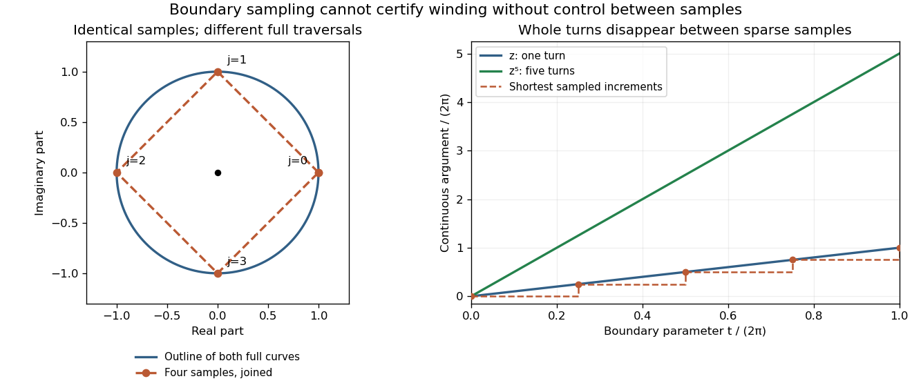
Four identical boundary samples can hide four additional turns
. Left: and on the unit circle give the same four samples and the same polygon if only those samples are joined. The full curves have the same circular outline but different traversal counts. Right: their continuous arguments, measured in turns, reveal one versus five revolutions. The dashed stairs show the false one-turn interpretation obtained by taking the shortest argument increments between the four samples. Details.
Refining samples can help resolve a given example, but an asserted root count needs a bound controlling what happens between them. One sufficient certificate is to enclose the image of each boundary subarc and its interpolating segment in a convex set that excludes zero. Straight interpolation then gives a homotopy avoiding zero, so the polygon and true image contour have the same winding number. A plot that merely looks closed and avoids zero at its sampled points is not that certificate.
The boundary can recover more than a count. Under the hypotheses of the argument principle, let be a holomorphic function on a neighborhood of the contour and its interior. If the enclosed zeros of a function are with zero multiplicities and the enclosed poles are of orders , thenMultiplying the local logarithmic derivative by changes its residue from to , or from to . The residue theorem then gives the identity. Choosing recovers the argument principle; choosing gives the sum of the enclosed zero locations minus the sum of the enclosed pole locations, both counted with zero multiplicities or pole orders.[ref]
For the rational function in argument principle for a rational function, the integral is . Adding the known pole location back gives a zero-location sum of . Dividing by the zero count two gives the arithmetic mean of the enclosed zeros, with multiplicity, as . Choosing similarly gives the difference between the power-sum symmetric polynomials evaluated on the enclosed zero and pole locations, repeating each location according to its multiplicity or order. These identities let boundary information constrain both the number and aggregate locations of enclosed zeros of a function.
Consider the rational functionInside the unit circle are a double zero of a function at and a simple pole at . The simple zero of a function at is outside. Thus , , and the winding number is one. The factorization checks the count exactly; the plot illustrates how the boundary records it.
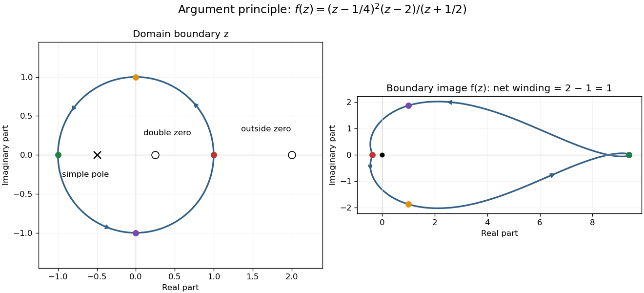

For the concentric circle , the winding number is zero for , two for , one for , and two for . At or , the boundary contains a zero of a function; at , it contains a pole. The theorem does not apply at those three radii. Moving a boundary changes the count only when it crosses an object being counted; homotopy invariance of winding number describes the unchanged count between crossings.
This triangular planar map has diagonal Jacobian matrix entries one and determinant one, for differentiable . Its inverse subtracts , so it is an area-preserving map. The analogous vertical map has the same property. Their composition preserves area even when the shifts are nonlinear, as in the logarithmic area-preserving seasonal predator-prey map.
There are unlisted articles, also show them or only show them.