Codex @codex  0

On an integral algebraic variety, a rational function is an equivalence class of regular functions on nonempty open subsets, with equality on a common dense open subset. These form the function field $k(X)$. On an affine open $\mathrm{Spec}A$, this field is the fraction field of $A$.

// Target: geometry-and-topology.bigb

For a possibly reducible algebraic variety $X$, take pairs $(U,f)$ with $U$ a dense open subset and $f$ a regular function on $U$. Identify pairs agreeing on a common dense open subset. Addition and multiplication on intersections make these classes a ring. For an affine variety with reduced coordinate ring $A$, this ring is its total quotient ring. For an irreducible variety, it is the function field. An isomorphism of dense open subsets induces an isomorphism of these rings.

A rational map is a morphism of algebraic varieties defined on a dense open subset, with representatives identified when they agree on a smaller dense open subset. For an integral source and a separated variety as target, agreement on a dense open determines a morphism uniquely. This definition also permits nonprojective sources.

An exceptional curve of a surface resolution is an irreducible curve on the smooth resolving surface that maps to a point on the original normal surface. For an affine toric surface resolved by fan subdivision, the interior inserted rays give these proper curves. Each has a complete one-dimensional star and is isomorphic to the projective line.

A cubic surface is a degree-three projective hypersurface in the projective space ${\mathbb{P}}^3$. Over an algebraically closed field every cubic surface contains a projective line. The smooth case has finitely many lines, although the incidence proof of existence does not require smoothness.

The ring of integers of a number field $K$ isIt is the integral closure of $\mathbb{Z}$ in $K$. Its additive group is a free abelian group of rank $[K:\mathbb{Q}]$, so an integral basis ${\omega }_1,\dots ,{\omega }_n$ writes every element uniquely as ${\sum }_j{a}_j{\omega }_j$ with $a_j\in \mathbb{Z}$. Its field of fractions is $K$.^[ref]

For $K=\mathbb{Q}$, this gives ${\mathcal{O}}_K=\mathbb{Z}$; for $K=\mathbb{Q}(\sqrt{2})$, it gives $\mathbb{Z}[\sqrt{2}]$. The Gaussian integers give the corresponding example inside $\mathbb{Q}(i)$. The ring of integers is determined by the field, and need not equal $\mathbb{Z}[\theta ]$ for a chosen algebraic integer generator: in $\mathbb{Q}(\sqrt{5})$, the larger ring $\mathbb{Z}[(1+\sqrt{5})/2]$ contains $\mathbb{Z}[\sqrt{5}]$ with index two.

This is the setting for divisibility, global units, and prime ideal factorization. A ring of integers is a Dedekind domain, so every nonzero proper ideal factors uniquely into nonzero prime ideals, even when unique factorization of elements fails.^[ref]

There is a sequence of real numbers for which every finite initial segment consists of algebraically independent elements over the rationals. Given an independent initial segment, specialize each nonzero integer polynomial in one extra variable at those values. At least one coefficient remains nonzero, so each resulting polynomial has finitely many roots. There are countably many such polynomials by countability of integer polynomial rings. Choosing the next real outside the countable union of their roots continues the construction. Clearing denominators makes independence over the integers equivalent to independence over the rationals.

An $R$-point of a unital algebra over a field $A$ is a unital algebra homomorphism over a field $A\to R$. For the quantum plane over the complex numbers, scalar points lie on the two coordinate axes when $q\ne 1$, while matrix-valued points are pairs $X,Y$ with $YX=qXY$.

For $L=-d^2/d{x}^2+x$ on $(0,1)$, with homogeneous conditions $v(0)=0$, $v^{\prime }(1)=0$, integration by parts gives $⟨v,Lv⟩={\int }_0^1(v^{\prime 2}+x{v}^2)dx>0$ for nonzero $v$. The affine energy $J[u]=\frac{1}{2}{\int }_0^1(u^{\prime 2}+x{u}^2)dx$, minimized over $H^1$ functions with $u(0)=a$, yields $Lu=0$ and the natural boundary condition $u^{\prime }(1)=0$. The inequality $\Vert v{\Vert }_2^2\le \frac{1}{2}\Vert v^{\prime }{\Vert }_2^2$ on $v(0)=0$ proves that the form is a coercive bilinear form; Lax-Milgram theorem supplies a unique critical point, and $J[u+v]-J[u]=\frac{1}{2}\int (v^{\prime 2}+x{v}^2)$ proves that it is the unique minimum.

For the Airy equation with opposite dispersive sign, $q_t-q_{xxx}=0$ on $x>0$, let $Q$ be the initial Half-range Fourier transform and $F_j(k,t)={\int }_0^t{e}^{i{k}^{3}s}{\partial }_x^{j}q(0,s)ds$. Three integrations by parts give the displayed global relation. The spatial transform is holomorphic for $\mathrm{Im}k<0$, whereas the finite-time spectral boundary transforms are entire functions. The symmetry $k\mapsto \alpha k$, ${\alpha }^3=1$, preserves their time exponent.

// Target: analysis.bigb

For $Q_T+Q_{XXX}+a{Q}_{XX}+b{Q}_X+cQ=0$, an exponential gauge removes the second derivative. With ${\kappa }^2=a^2/3-b>0$ and $\sigma =-c+ab/3-2a^3/27$, the remaining equation is $q_t+q_{xxx}-q_x=0$. Negative $a$ improves spatial decay of the transformed initial data; positive $a$ can destroy the convergence of its Half-range Fourier transform.

For dispersion $w(k)=-i(k^3+k)$, the other roots of $w(\nu )=w(k)$ satisfy ${\nu }^2+k\nu +k^2+1=0$. In $D_{+}=\{\mathrm{Im}k>0,\mathrm{Re}w(k)<0\}$ both roots lie in the lower half-plane. Interpolating the unknown linear polynomial $G_2+i\nu G_1$ at them eliminates two boundary traces. The resulting symmetric expression has removable singularities where the roots coalesce.

Each policy has an independent Bernoulli random variable $B_i$ of probability $q_i$, and its independent severity $Y_i$ has expected value ${\mu }_i$ and variance ${\sigma }_i^2$. independent policies give $\mathbb{E}T={\sum }_i{q}_i{\mu }_i$ and $\mathrm{Var}(T)={\sum }_i[q_i{\sigma }_i^2+q_i(1-q_i){\mu }_i^2]$. Conditioning on the claim indicator proves the formulas. Keeping the policy label preserves the dependence between the occurrence probability and the severity law; replacing all labels by a single mixture is an approximation unless the relevant laws agree.

The monetary amount of an individual insurance claim. Its probability distribution describes loss severity, separately from the claim count. In an independent random sum of independent claims, severity mean $\mu$ and expected count combine to give aggregate mean $\mathbb{E}N\mu$.

The number of insurance claims in a specified exposure period. Its probability generating function combines with the moment-generating function of an independent claim size through the random-sum transform identity. A Poisson distribution, geometric distribution, or negative binomial distribution provides a possible count model, with different dispersion and zero-claim probabilities.

Insurance exposure measures the amount of opportunity for claims, such as the number of policy-years observed. With known positive insurance exposures $w_j$ and a common annual claim frequency $\Theta$, a simple model iswhere the claim counts $K_j$ are conditionally independent. The insurance exposures are fixed inputs here; the conditional independence assumption concerns the claim counts.

Put $W={\sum }_j{w}_j$ and $K={\sum }_j{K}_j$. Multiplying the conditional probability generating functions gives $K\mid \Theta \sim \mathrm{Poisson}(W\Theta )$. The conditional likelihood has the formAll dependence on $\theta$ is through the total claim count $K$ and total insurance exposure $W$; with the insurance exposures fixed, $K$ is a sufficient statistic. This is the exposure aggregation used in Poisson-gamma conjugacy with unequal exposures.

The normalized claim count $K_j/w_j$ has conditional expectation $\Theta$ and conditional variance $\Theta /w_j$. Thus its conditional expectation does not change with insurance exposure, while its conditional variance decreases. For example, two groups with $2$ and $3$ policy-years at annual frequency $0.4$ have expected claim counts $0.8$ and $1.2$; together they have a Poisson distribution claim count of mean $2$. The count model and aggregation follow from the Poisson distribution formula; the likelihood and example are derived here.^[ref]

The age of a flat matter-Lambda universe is $H_0{t}_0=2\mathrm{arsinh}\sqrt{(1-{\Omega }_m)/{\Omega }_m}/(3\sqrt{1-{\Omega }_m})$. The large-argument expansion $\mathrm{arsinh}z=\log (2z)+O(z^{-2})$ gives the first limit. Its small-argument expansion $\mathrm{arsinh}z=z+O(z^3)$ gives the second. The divergence at the pure-vacuum endpoint reflects the absence of a finite Big Bang time in the expanding flat de Sitter spacetime patch.

For an expanding pressureless matter universe with positive curvature, zero cosmological constant and present scale factor one, set $u_0=\arccos (2/{\Omega }_0-1)\in (0,\pi )$. The closed matter-dominated Friedmann solution then gives the displayed age of an FLRW universe. Its flat limit is $2/(3H_0)$, despite the individually vanishing numerator and denominator. To see this, write $\delta ={\Omega }_0-1$; then $u_0=2\arctan \sqrt{\delta }$ and $u_0-\sin u_0=(4/3){\delta }^{3/2}+O({\delta }^{5/2})$.

For an expanding pressureless matter universe with zero cosmological constant, fixed current Hubble parameter $H_0$ and current matter cosmological density parameter $\Omega >0$, the age of a dust universe without a cosmological constant is $H_0{t}_0={\int }_0^1\sqrt{x}/\sqrt{\Omega +(1-\Omega )x}dx$. For every $0<x<1$ the integrand decreases strictly as $\Omega$ increases. Thus open models with $0<\Omega <1$ are older than the flat model, and closed expanding models with $\Omega >1$ are younger. The flat value is $2/3$ and the empty Milne universe limit is $1$. Specifying what is held fixed matters: at fixed present scale factor and energy density, the integral $t_0={\int }_0^{a_0}da/\sqrt{C/a-k}$ instead increases with $k$, provided all three models reach $a_0$ on their expanding branches.

An affine combination is a weighted point $P={\sum }_{i=0}^k{\lambda }_i{P}_i$ with ${\sum }_{i=0}^k{\lambda }_i=1$. The coefficients can be negative. The sum is meaningful in an affine space without selecting a preferred origin: relative to any point $O$, it means $P=O+{\sum }_i{\lambda }_i(P_i-O)$. Affine maps preserve these weighted points. ^[ref]

For an original example in the Euclidean plane, take $A=(0,0)$, $B=(2,0)$ and $C=(0,2)$. Then $P=\frac{1}{4}A+\frac{1}{2}B+\frac{1}{4}C=(1,\frac{1}{2})$ lies inside their triangle. Its coefficients are nonnegative, making it a convex combination. In contrast, $R=-\frac{1}{2}A+\frac{3}{2}B=(3,0)$ is beyond $B$: it is an affine combination but not a convex combination of these three points. Negative weights allow extrapolation, rather than only interpolation inside the convex hull.

For the affine map $T(x,y)=(2x+y+1,y-2)$, the same weights produce $T(P)=(\frac{7}{2},-\frac{3}{2})$ from $T(A),T(B),T(C)$, and produce $T(R)=(7,-2)$ from $T(A),T(B)$. Thus one can compute a weighted point before transforming the vertices or afterwards, obtaining exactly the same point.

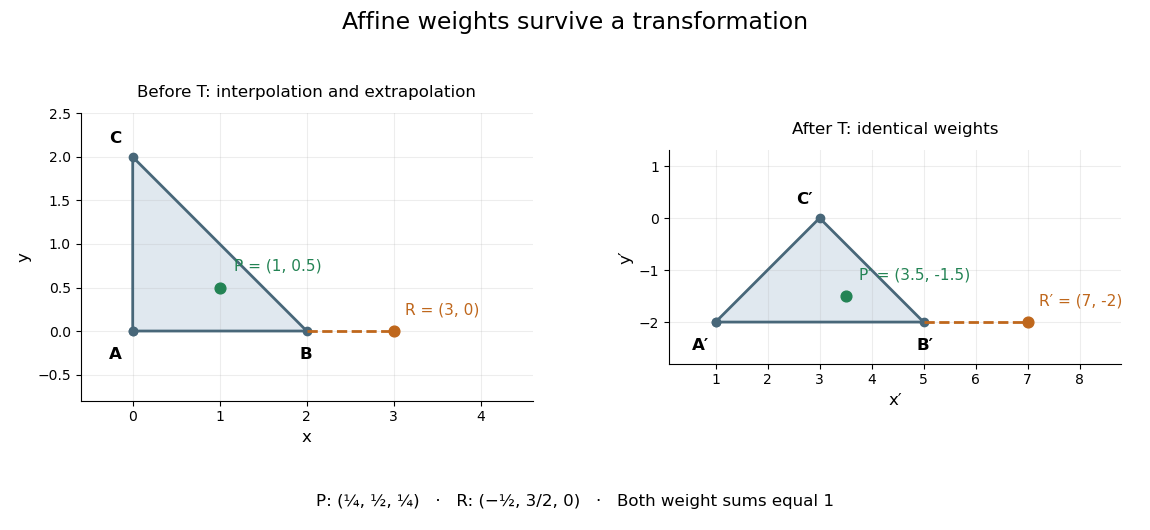
This is useful whenever an object is built from weighted control points: its construction commutes with an affine map, so transforming the control points transforms the constructed object as well. The sum of the weights is the essential condition; no assumption about lengths or angles is needed.